12-regression

Professor Shannon Ellis

UC San Diego
COGS 137 - Fall 2024

2024-11-14

Q&A

Q: kind of zoned out. When is it appropriate to use inference or machine learning?
A: We use inference when we want to quantify the relationship between features and outcome to understand relationships. We use machine learning when we want to make predictions on outcomes from features.

Q: I am confused why in EDA, we have been finding the correlation between variables that seem to be measuring the same thing (such as graphs for log distance to primary or primary and secondary road). Why are these helpful to us?
A: We are ultimately trying to build a model to predict PM2.5 values…but we have a lot of features from which to choose, many which measure very siimilar things. We’re using EDA to get a sense of what data we have and the relationships between variables, before ultimately deciding what to include in our ML model.

Course Announcements

Due Dates

🧪 Lab 06 due Thursday
📋 Lecture Participation survey “due” after class

Notes

lab05 scores posted; cs01 scores/feedback posted by EOD
lab07 now available | longer than typical labs
Reminder to add any CS02 EDA you want to share with your classmates to the padlet from last class

Agenda

Simple linear regression (review)
Multiple linear regression
Model Comparison
Backward Selection

Linear Regression

Setup

library(tidyverse)
library(tidymodels)
library(olsrr) # will need to be installed

Data

pm <- read_csv("OCS_data/data/raw/pm25_data.csv")

Rows: 876 Columns: 50
── Column specification ────────────────────────────────────────────────────────
Delimiter: ","
chr  (3): state, county, city
dbl (47): id, value, fips, lat, lon, CMAQ, zcta, zcta_area, zcta_pop, imp_a5...

ℹ Use `spec()` to retrieve the full column specification for this data.
ℹ Specify the column types or set `show_col_types = FALSE` to quiet this message.

Starting Question

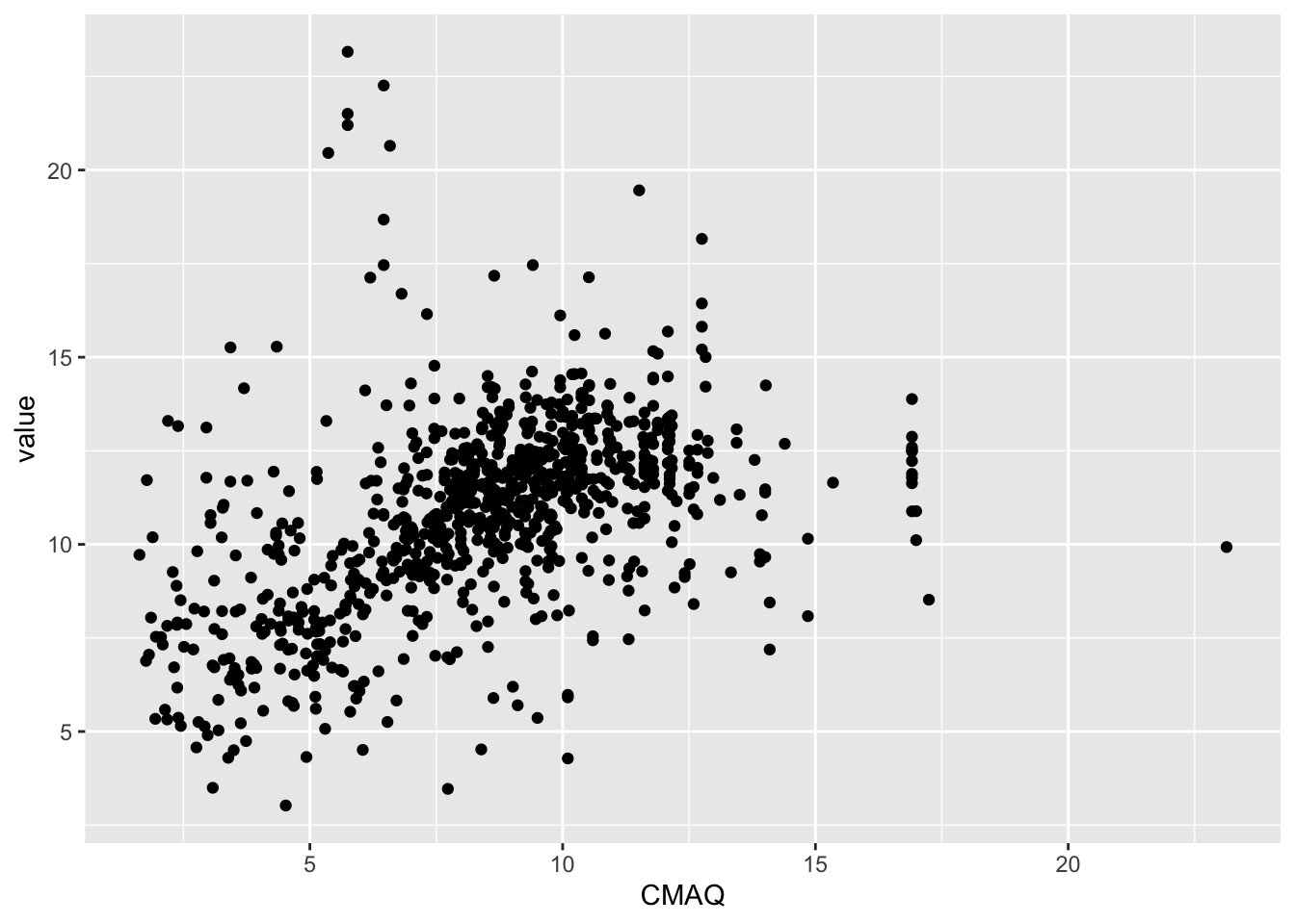
What is the relationship between the EPA’s CMAQ and PM2.5 values?

Reminder: Community Multiscale Air Quality (CMAQ) is the EPA’s air pollution model. The data do NOT use PM2.5 measures

Quick Look

ggplot(pm, aes(x=CMAQ, y=value)) + 
  geom_point()

Single predictor

Regression model

\[ \hat{y} = b_0 + b_1~x_1 \]

\(\hat{y}\) | outcome
\(x_1\) | predictor
\(b_0\) | y-intercept
\(b_1\) | slope (effect size)

Step 1: Specify model

linear_reg()

Linear Regression Model Specification (regression)

Computational engine: lm

Step 2: Set model fitting engine

lin_mod <- linear_reg() |>
  set_engine("lm") # lm: linear model

Step 3: Fit model & estimate parameters

… using formula syntax

# fit model
mod_cmaq_value <- lin_mod |>
  fit(value ~ CMAQ, data = pm) 

# display results
mod_cmaq_value |>
  tidy()

# A tibble: 2 × 5
  term        estimate std.error statistic   p.value
  <chr>          <dbl>     <dbl>     <dbl>     <dbl>
1 (Intercept)    7.40     0.232       31.9 1.81e-148
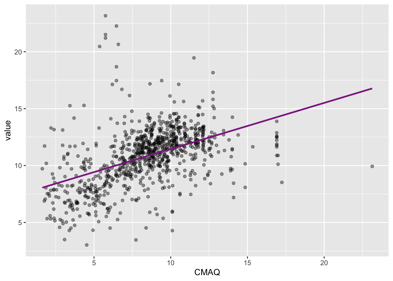
2 CMAQ           0.405    0.0260      15.6 1.83e- 48

\[\widehat{PM2.5}_{i} = 7.40 + 0.405 \times CMAQ_{i}\]

Visualizing the model

ggplot(data = pm, aes(x = CMAQ, y = value)) +
  geom_point(alpha = 0.4) +
  geom_smooth(method = "lm", fullrange = TRUE, color = "#8E2C90", se = FALSE)

Slope and intercept

\[\widehat{PM2.5}_{i} = 7.40 + 0.405 \times CMAQ_{i}\]

Slope: For each one unit increase in CMAQ, we expect PM2.5 to increase, on average, by 0.405 ug/m^3.

Intercept: Monitors in areas with a CMAQ of zero are expected to have PM2.5 values of 7.4 ug/m^3, on average. (Recall: WHO exposure guideline is < 10 ug/m^3 on average annually for PM2.5)

Model Understanding

\[\widehat{PM2.5}_{i} = 7.40 + 0.405 \times CMAQ_{i}\]

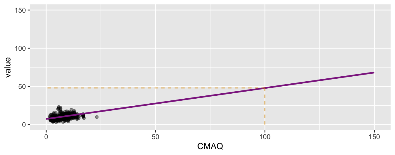
❓ What would we expect the PM2.5 value to be in an area with a CMAQ of 2?

❗️Prediction vs. extrapolation

❓ What would we expect the PM2.5 value to be in an area with a CMAQ of 100? \[\widehat{PM2.5}_{i} = 7.40 + 0.405 \times 100\]

Measuring the strength of the fit

The strength of the fit of a linear model is most commonly evaluated using \(R^2\).
It tells us what percent of variability in the response variable is explained by the model.
The remainder of the variability is explained by variables not included in the model.
\(R^2\) is sometimes called the coefficient of determination.

Obtaining \(R^2\) in R

glance(mod_cmaq_value)

# A tibble: 1 × 12
  r.squared adj.r.squared sigma statistic  p.value    df logLik   AIC   BIC
      <dbl>         <dbl> <dbl>     <dbl>    <dbl> <dbl>  <dbl> <dbl> <dbl>
1     0.217         0.216  2.29      243. 1.83e-48     1 -1966. 3939. 3953.
# ℹ 3 more variables: deviance <dbl>, df.residual <int>, nobs <int>

glance(mod_cmaq_value)$r.squared # extract R-squared

[1] 0.2172969

Roughly 21.7% of the variability in PM2.5 values can be explained by CMAQ.

…suggests that we can do better to explain the variance in PM2.5 values

Multiple predictors (MLR)

MLR

Sample model that we use to estimate the population model:

\[ \hat{y} = b_0 + b_1~x_1 + b_2~x_2 + \cdots + b_k~x_k \]

Updated question

What is the relationship between CMAQ & population density (predictors) and and PM2.5 values (outcome)?

Response variable: value (PM2.5)
Explanatory variables: CMAQ and Population Density hi/low

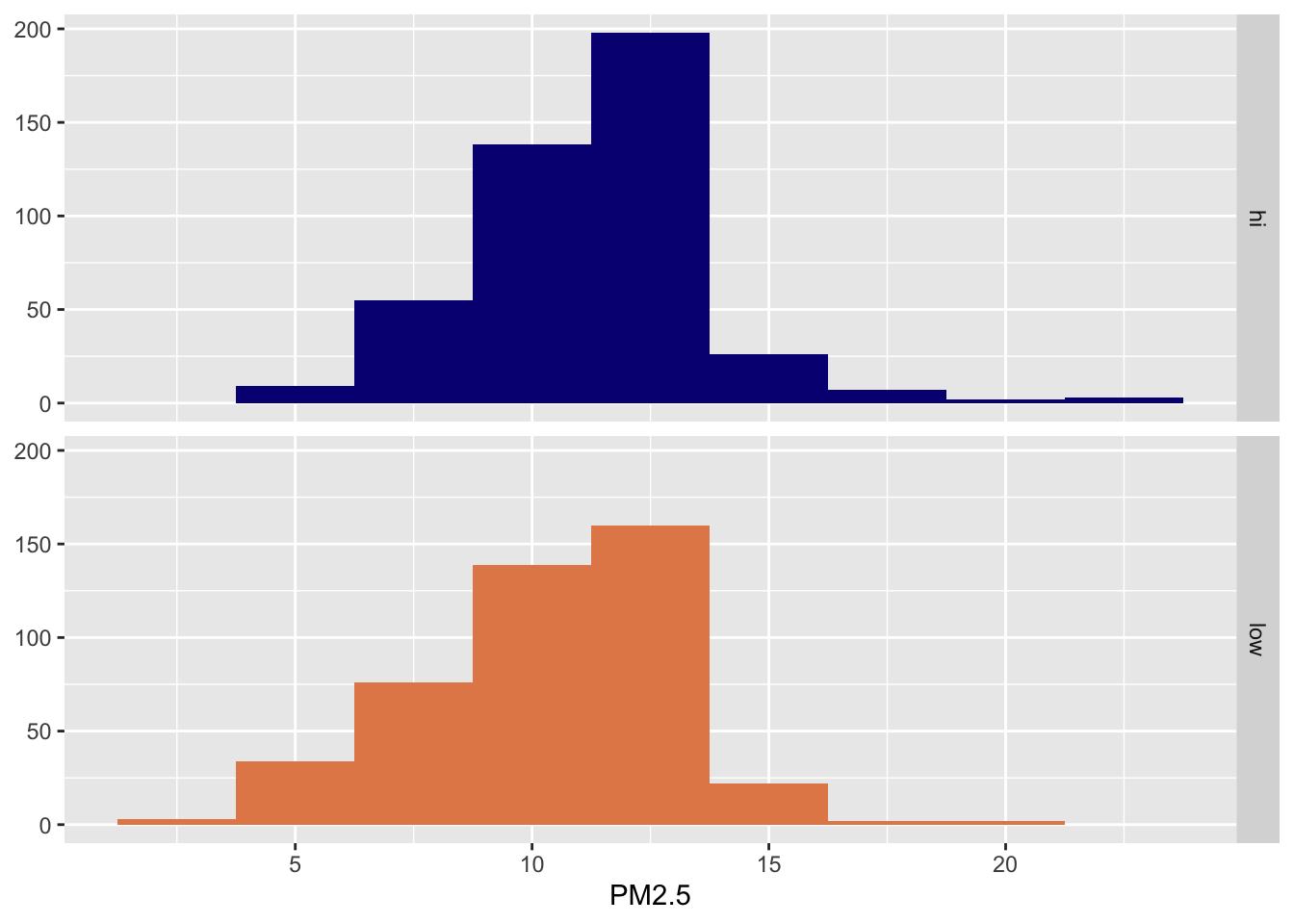
Creating a low/high population density variable

pm <- pm |> 
  mutate(popdens = case_when(
    popdens_zcta >= median(pm$popdens_zcta) ~ "hi",
    popdens_zcta < median(pm$popdens_zcta) ~ "low"          
  ))

❓ What is this accomplishing?

ggplot(data = pm, aes(x = value, fill = popdens)) +
  geom_histogram(binwidth = 2.5) + 
  facet_grid(popdens ~ .) +
  scale_fill_manual(values = c("#071381", "#E48957")) +
  guides(fill = "none") +
  labs(x = "PM2.5", y = NULL)

Two ways to model

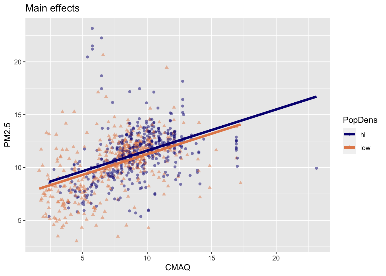
Main effects: Assuming relationship between CMAQ and PM2.5 does not vary by whether it’s a low or high population density monitor.
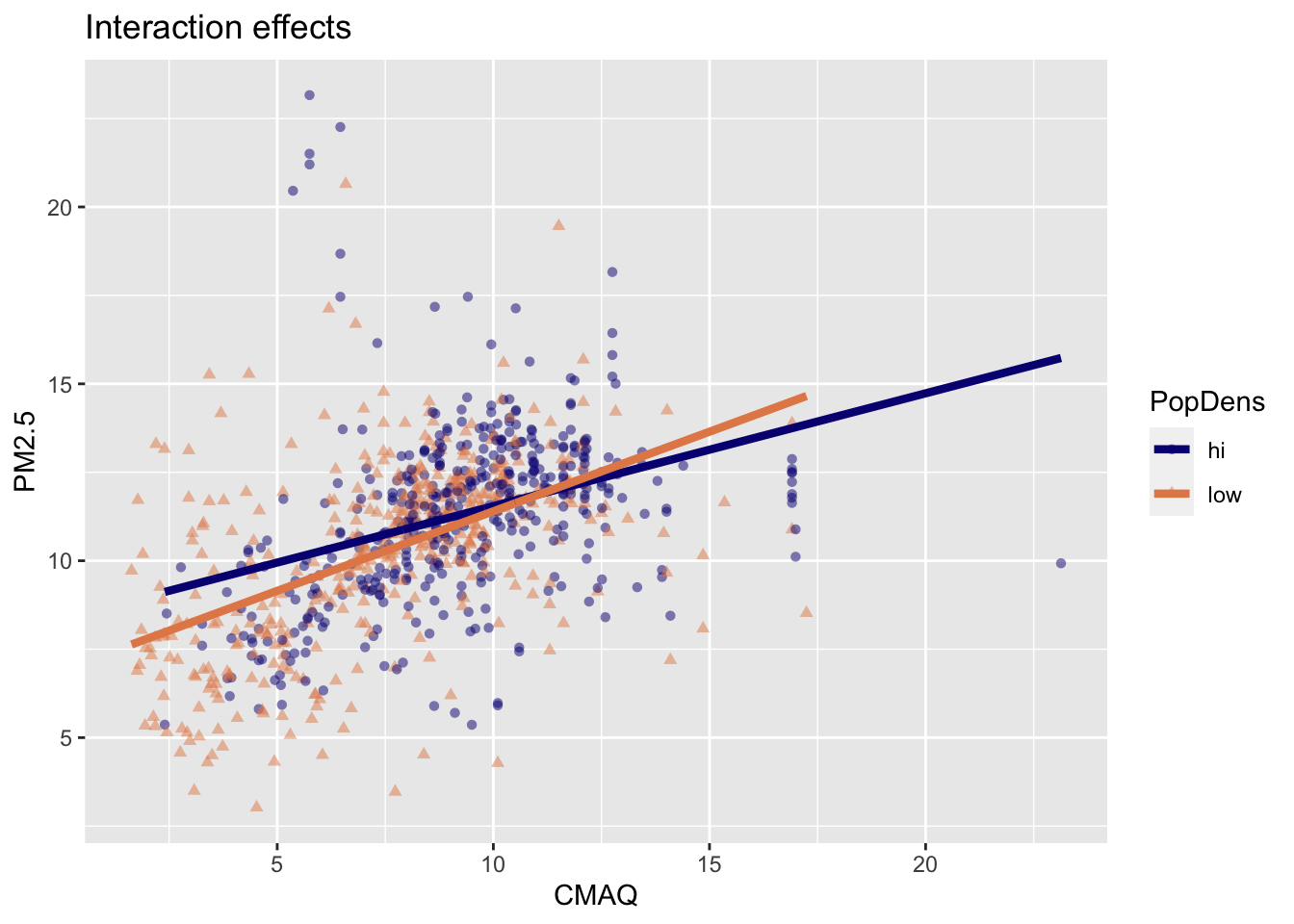
Interaction effects: Assuming relationship between CMAQ and PM2. varies by whether or not it’s a low or high population density monitor.

Interacting explanatory variables

Including an interaction effect in the model allows for different slopes, i.e. nonparallel lines.
This implies that the regression coefficient for an explanatory variable would change as another explanatory variable changes.
This can be accomplished by adding an interaction variable: the product of two explanatory variables.

Two ways to model

Main effects: Assuming relationship between CMAQ and PM2.5 does not vary by whether it’s a low or high population density monitor.
Interaction effects: Assuming relationship between CMAQ and PM2. varies by whether or not it’s a low or high population density monitor.

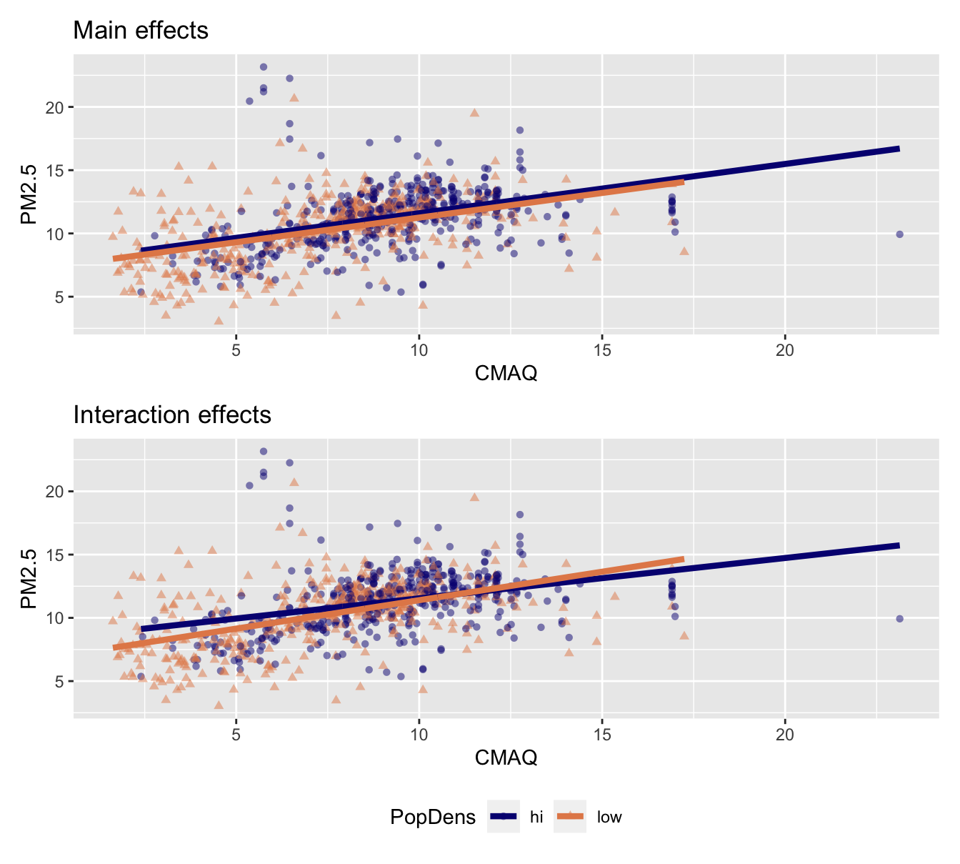
❓ Which does your intuition/knowledge of the data suggest is more appropriate?

Put a green sticky if you think main; pink if you think interaction.

Fit model with main effects

pm_main_fit <- lin_mod |>
  fit(value ~ CMAQ + popdens, data = pm)

pm_main_fit |> tidy()

# A tibble: 3 × 5
  term        estimate std.error statistic   p.value
  <chr>          <dbl>     <dbl>     <dbl>     <dbl>
1 (Intercept)    7.70     0.272      28.3  1.02e-125
2 CMAQ           0.389    0.0270     14.4  1.89e- 42
3 popdenslow    -0.345    0.160      -2.15 3.17e-  2

\[\widehat{PM2.5} = 7.70 + 0.389 \times CMAQ - 0.345 \times popdens\]

❓ How do we interpret this model?

Solving the model

High-population density: Plug in 0 for popdens

\[\widehat{PM2.5} = 7.70 + 0.389 \times CMAQ - 0.345 \times 0\]
\(= 7.70 + 0.389 \times CMAQ\)

Low-population density: Plug in 1 for popdens

\[\widehat{PM2.5} = 7.70 + 0.389 \times CMAQ - 0.345 \times 1\]
\(= 7.355 + 0.389 \times CMAQ\)

Visualizing main effects

Same slope: Rate of change in PM2.5 as CMAQ increases does not vary between low- and high-population density monitor areas.
Different intercept: Areas of low density have consistently lower PM2.5 values relative to high-population density areas

Interpreting main effects

pm_main_fit |>
  tidy() |> 
  mutate(exp_estimate = exp(estimate)) |>
  select(term, estimate, exp_estimate)

# A tibble: 3 × 3
  term        estimate exp_estimate
  <chr>          <dbl>        <dbl>
1 (Intercept)    7.70      2217.   
2 CMAQ           0.389        1.48 
3 popdenslow    -0.345        0.708

All else held constant, for each 1 unit increase in CMAQ, PM2.5 would expect to increase by 0.389.
All else held constant, areas of low density have PM2.5 values, on average, that are 0.345 lower than in high density areas
PM2.5 values in high-density areas with a CMAQ of zero, would expect to have a PM2.5 value of 7.7.

Interaction: `CMAQ * popdens`

Fit model with interaction effects

Response variable: value (PM2.5)
Explanatory variables: CMAQ, popdens, and their interaction

pm_int_fit <- lin_mod |>
  fit(value ~ CMAQ * popdens, data = pm)

Linear model with interaction effects

# A tibble: 4 × 5
  term            estimate std.error statistic  p.value
  <chr>              <dbl>     <dbl>     <dbl>    <dbl>
1 (Intercept)        8.35     0.381      21.9  4.63e-85
2 CMAQ               0.319    0.0396      8.05 2.69e-15
3 popdenslow        -1.45     0.485      -3.00 2.79e- 3
4 CMAQ:popdenslow    0.131    0.0540      2.42 1.56e- 2

\[\widehat{PM2.5} = 8.35 + 0.32 \times CMAQ - 1.45 \times popdens + 0.13 \times CMAQ * popdens\]

Interpretation of interaction effects

Rate of change in PM2.5 as CMAQ increases varies depending upon PopDens (different slopes & intercepts)

Comparing models

R-squared

\(R^2\) is the percentage of variability in the response variable explained by the regression model.

glance(mod_cmaq_value)$r.squared #single predictor

[1] 0.2172969

glance(pm_main_fit)$r.squared

[1] 0.2214237

glance(pm_int_fit)$r.squared

[1] 0.2266283

The model with interactions has a slightly higher \(R^2\).

However using \(R^2\) for model selection in models with multiple explanatory variables is not a good idea as \(R^2\) increases when any variable is added to the model.

Adjusted R-squared

Adjusted R-squared adjusts for number of terms in the model

glance(pm_main_fit)$adj.r.squared

[1] 0.21964

glance(pm_int_fit)$adj.r.squared

[1] 0.2239676

It appears that adding the interaction actually increased adjusted \(R^2\), so we should indeed use the model with the interactions.

In pursuit of Occam’s razor

Occam’s Razor states that among competing hypotheses that predict equally well, the one with the fewest assumptions should be selected.
Model selection follows this principle.
We only want to add another variable to the model if the addition of that variable brings something valuable in terms of predictive power to the model.
In other words, we prefer the simplest best model, i.e. parsimonious model.

Backward selection

For this demo, we’ll ignore interaction effects…and just model main effects:

pm_full <-  lin_mod |>
  fit(value ~ ., data=pm)

\(R^2\) (full): 0.9125688

Remove zcta_area

pm_noarea <-  lin_mod |>
  fit(value ~ . -zcta_area, data=pm) 

glance(pm_noarea)$adj.r.squared

[1] 0.9134989

\(R^2\) (full): 0.9126
\(R^2\) (no zcta_area): 0.9135

…Increased improved variance explained, so remove variable

… continue to remove one by one until max variance explained is achieved. But, that process is tedious.

Other approach: `olsrr`

# requires package installation: 
# install.packages("olsrr")
library(olsrr)

Step 1: Fit full model (w/o tidymodels)

Note: I’m only fitting a handful of variables to demo how it works. Theoretically, you would fit the full model and compare all combinations.

# fit the model (not using tidymodels)
mod <- lm(value ~ log_pri_length_25000 + log_prisec_length_15000 +
          log_nei_2008_pm25_sum_15000 , data=pm)

Step 2: Determine which variables to remove

ols_step_backward_p(mod)


                                 Elimination Summary                                  
-------------------------------------------------------------------------------------
        Variable                              Adj.                                       
Step          Removed           R-Square    R-Square     C(p)        AIC        RMSE     
-------------------------------------------------------------------------------------
   1    log_pri_length_25000      0.1643      0.1624    2.3628    3998.1896    2.3638    
-------------------------------------------------------------------------------------

…specifies that log_pri_length_25000 should be removed

Step 2 (alternate): Compare all possible models…

ols_step_all_possible(mod) |>
  arrange(desc(adjr))

  Index N
1     4 2
2     7 3
3     5 2
4     1 1
5     2 1
6     6 2
7     3 1
                                                                Predictors
1                      log_prisec_length_15000 log_nei_2008_pm25_sum_15000
2 log_pri_length_25000 log_prisec_length_15000 log_nei_2008_pm25_sum_15000
3                         log_pri_length_25000 log_nei_2008_pm25_sum_15000
4                                              log_nei_2008_pm25_sum_15000
5                                                  log_prisec_length_15000
6                             log_pri_length_25000 log_prisec_length_15000
7                                                     log_pri_length_25000
    R-Square Adj. R-Square Mallow's Cp
1 0.16433852    0.16242406    2.362832
2 0.16468608    0.16181230    4.000000
3 0.13894927    0.13697665   28.867142
4 0.12833737    0.12734004   37.945112
5 0.12004781    0.11904100   46.598742
6 0.12047519    0.11846024   48.152590
7 0.06827606    0.06721001  100.644250

On the full model

This will take a while to run:

mod_full <- lm(value ~ ., data=pm)
ols_step_backward_p(mod_full)


                                      Elimination Summary                                       
-----------------------------------------------------------------------------------------------
        Variable                                     Adj.                                          
Step              Removed              R-Square    R-Square      C(p)          AIC        RMSE     
-----------------------------------------------------------------------------------------------
   1    zcta_area                        0.9907      0.9135    -686.9999    2393.0696    0.7597    
   2    imp_a10000                       0.9907      0.9144    -688.9885    2391.1777    0.7557    
   3    imp_a15000                       0.9907      0.9153    -690.9804    2389.2532    0.7518    
   4    popdens                          0.9907      0.9161    -692.9669    2387.3804    0.7479    
   5    lon                              0.9907       0.917    -694.9512    2385.5282    0.7442    
   6    log_nei_2008_pm25_sum_25000      0.9907      0.9178    -696.9317    2383.7123    0.7405    
   7    log_pri_length_5000              0.9907      0.9186    -698.8475    2382.5047    0.7371    
   8    pov                              0.9907      0.9193    -700.7333    2381.5780    0.7339    
   9    log_dist_to_prisec               0.9907      0.9199    -702.5666    2381.1422    0.7310    
  10    log_prisec_length_5000           0.9906      0.9205    -704.3919    2380.7786    0.7281    
  11    imp_a5000                        0.9906      0.9212    -706.2355    2380.2407    0.7252    
  12    id                               0.9906      0.9216    -707.8749    2381.6028    0.7231    
  13    log_prisec_length_1000           0.9906       0.922    -709.4443    2383.6011    0.7213    
  14    county_area                      0.9905      0.9224    -710.9958    2385.7466    0.7196    
  15    popdens_county                   0.9904      0.9226    -712.3595    2389.5945    0.7187    
  16    county_pop                       0.9904      0.9226    -713.5295    2395.1638    0.7185    
  17    log_prisec_length_10000          0.9903      0.9226    -714.6346    2401.2525    0.7185    
  18    log_pri_length_10000             0.9902      0.9229    -716.1117    2403.9439    0.7172    
  19    log_pri_length_15000             0.9901       0.923    -717.4012    2408.2793    0.7166    
-----------------------------------------------------------------------------------------------

❓ How does this maybe inform our ultimate goal (building a prediction model)?

Recap

Can you model and interpret linear models with multiple predictors?
Can you explain the difference in a model with main effects vs. interaction effects?
Can you compare different models and determine how to proceed?
Can you carry out and explain backward selection?

12-regression

Q&A

Course Announcements

Agenda

Suggested Reading

Linear Regression

Setup

Data

Starting Question

Quick Look

Single predictor

Regression model

Step 1: Specify model

Step 2: Set model fitting engine

Step 3: Fit model & estimate parameters

Visualizing the model

Slope and intercept

Model Understanding

❗️Prediction vs. extrapolation

Measuring the strength of the fit

Obtaining \(R^2\) in R

Multiple predictors (MLR)

MLR

Updated question

Creating a low/high population density variable

PM2.5 & Poulation density

Two ways to model

Interacting explanatory variables

Two ways to model

Fit model with main effects

Solving the model

Visualizing main effects

Interpreting main effects

Interaction: CMAQ * popdens

Fit model with interaction effects

Linear model with interaction effects

Interpretation of interaction effects

Comparing models

R-squared

Adjusted R-squared

In pursuit of Occam’s razor

Backward selection

Backward selection

Other approach: olsrr

On the full model

Recap

Interaction: `CMAQ * popdens`

Other approach: `olsrr`