03-dplyr

Author

Affiliation

Professor Shannon Ellis

UC San Diego
COGS 137 - Fall 2024

Published

October 8, 2024

Data Manipulation with `dplyr`

[ad] EDGE

Mentorship opportunity for women-identifying students:

Q&A

Q: what does |> mean? Do we need to know a lot of how to code those examples from class?
A: Love that you’re noting and questioning these things. We’re going to discuss this today! You do not need to know the code examples…yet. We’re going to discuss code starting today; this starts with what you’ll need to be familiar with.

Q: How to really extend the case study in our own time, when many information/analysis are already given in the lecture?
A: We’ll discuss this more! But, specifically for this first Case Study. We’re asking a very narrow question….but have a lot of variables. Is there some subgroup you could focus on? A different time window? A combination of compounds? Etc.

Q: How can we do more complex math in R?
A: Depends on what kind of complex math you’re aiming to do - a lot of complex math is built directly into R; other things would require additional packages.

Q: Where can I find the full study on the data we reviewed in class. Seems like something I’d like to read and perhaps play with the data myself.
A: We’re going to discuss the results today! But, the links are inlcuded in the notes (in what we didn’t get to yet.)

Q: How did the police officers do to detect cognitive impariedness with marijuana consumption?
A: Not great (not better than flipping a coin). We’ll discuss this today!

Q: Why were the numeric types in the cat lovers data frame labeled as ‘dbl’ instead of numeric?
A: There are multiple “levels” of object type in R (which I did not make clear in lecture b/c it’s not important for this class). Double is a subset of numeric. If you ask for type() rather than class() you’ll see this difference.

Q: In class, we used |> as a pipe operator. Is it fine if we use %>% instead? Do you have a preference between the two? Thank you!
A: We’ll discuss this today - no preference!

Q: My github username is pretty weird. How are the professor and TA going to know that it is me if my username does not resemble my actual name?
A: On your first lab, we ask you to put your name in the author field. We use that to match students to their GH usernames!

Course Announcements

Due Dates:

Lab 01 due Thursday (10/10 11:59 PM; push to GH)
HW01 now available; due Monday (10/14; 11:59 PM)
Lecture Participation survey “due” after class

. . .

Notes:

No Lecture on Thursday this week
Discuss: GH<->RStudio issue (OpenSSL version mismatch. Built against 30000020, you have 30300020)
Regular labs resume this week
Mention: waitlist & dropping

Agenda

dplyr
- philosophy
- pipes
- common operations
CS01 Wrangling

Philosophy

dplyr is a grammar of data manipulation, providing a consistent set of verbs that help you solve the most common data manipulation challenges

Source: dplyr.tidyverse.org

Pipes

The pipe in baseR

|> should be read as “and then”
for example “Wake up |> brush teeth” would be read as “wake up and then brush teeth”

Where does the name come from?

The pipe operator was first implemented in the package magrittr.

You will see this frequently in code online. It’s equivalent to |>.

How does a pipe work?

You can think about the following sequence of actions - find key, unlock car, start car, drive to school, park.

. . .

Expressed as a set of nested functions in R pseudocode this would look like:

park(drive(start_car(find("keys")), to = "campus"))

. . .

Writing it out using pipes give it a more natural (and easier to read) structure:

find("keys") |>
  start_car() |>
  drive(to = "campus") |>
  park()

. . .

(Reminder to comment on indentation/alignment)

Data

To get started with lecture code: library(tidyverse)

Whole Blood (WB) Data from THC Study

WB <- read_csv("https://github.com/ShanEllis/datasets/raw/refs/heads/master/Blood.csv")

Important

We’re using these data to demonstrate the basic principles of dplyr and tidyr before we get to how to specifically clean our CS01 data.

. . .

Read the data in so you can follow along now!

Put a green sticky on the front of your computer when you’re done. Put a pink if you want help/have a question.

Variables

View the names of variables via:

names(WB)

 [1] "ID"              "Treatment"       "Group"           "FLUID TYPE"     
 [5] "Timepoint"       "CBN"             "CBD"             "THC"            
 [9] "11-OH-THC"       "THC-COOH"        "THC-COOH-Gluc"   "CBG"            
[13] "THC-V"           "time.from.start"

Viewing your data

In the Environment, click on the name of the data frame to view it in the data viewer (or use the View function)
Use the glimpse function to take a peek

glimpse(WB)

Rows: 1,525
Columns: 14
$ ID              <chr> "11255", "11255", "11255", "11255", "11255", "11255", …
$ Treatment       <chr> "5.90%", "5.90%", "5.90%", "5.90%", "5.90%", "5.90%", …
$ Group           <chr> "Occasional user", "Occasional user", "Occasional user…
$ `FLUID TYPE`    <chr> "WB", "WB", "WB", "WB", "WB", "WB", "WB", "WB", "WB", …
$ Timepoint       <chr> "T1", "T2A", "T2B", "T3A", "T3B", "T4A", "T4B", "T5A",…
$ CBN             <dbl> 0.0, 2.8, 0.6, 0.0, 0.0, 0.0, 0.0, 0.0, 0.0, 0.0, 4.6,…
$ CBD             <dbl> 0, 0, 0, 0, 0, 0, 0, 0, 0, 0, 0, 0, 0, 0, 0, 0, 0, 0, …
$ THC             <dbl> 0.5, 32.4, 5.1, 3.2, 1.8, 1.2, 0.9, 0.8, 0.6, 0.0, 46.…
$ `11-OH-THC`     <dbl> 0.0, 5.4, 2.4, 1.8, 1.4, 0.0, 0.0, 0.0, 0.0, 0.0, 7.7,…
$ `THC-COOH`      <dbl> 5.7, 13.5, 11.7, 9.7, 8.7, 6.7, 6.8, 6.8, 6.3, 1.9, 13…
$ `THC-COOH-Gluc` <dbl> 4.9, 4.4, 6.2, 8.4, 8.9, 8.2, 7.5, 7.1, 6.1, 2.1, 2.7,…
$ CBG             <dbl> 0.0, 1.2, 0.0, 0.0, 0.0, 0.0, 0.0, 0.0, 0.0, 0.0, 2.0,…
$ `THC-V`         <dbl> 0, 0, 0, 0, 0, 0, 0, 0, 0, 0, 0, 0, 0, 0, 0, 0, 0, 0, …
$ time.from.start <dbl> -27, 15, 69, 111, 156, 236, 283, 315, 360, -10, 20, 73…

`dplyr`

A Grammar of Data Manipulation

dplyr is based on the concepts of functions as verbs that manipulate data frames.

Single data frame functions / verbs:

filter: pick rows matching criteria
mutate: add new variables
select: pick columns by name
rename: rename specific columns
summarize: reduce variables to values
arrange: reorder rows
distinct: filter for unique rows
pull: grab a column as a vector
sample_n / sample_frac: randomly sample rows
slice: pick rows using index(es)
… (many more)

`dplyr` rules for functions

First argument is always a data frame
Subsequent arguments say what to do with that data frame
Always return a data frame
Do not modify in place
Performance via lazy evaluation

Filter rows with `filter`

Select a subset of rows in a data frame.
Easily filter for many conditions at once.

`filter` (single condition)

for only measurements from Occasional users

WB |>
  filter(Group == "Occasional user")

# A tibble: 750 × 14
   ID    Treatment Group    `FLUID TYPE` Timepoint   CBN   CBD   THC `11-OH-THC`
   <chr> <chr>     <chr>    <chr>        <chr>     <dbl> <dbl> <dbl>       <dbl>
 1 11255 5.90%     Occasio… WB           T1          0       0   0.5         0  
 2 11255 5.90%     Occasio… WB           T2A         2.8     0  32.4         5.4
 3 11255 5.90%     Occasio… WB           T2B         0.6     0   5.1         2.4
 4 11255 5.90%     Occasio… WB           T3A         0       0   3.2         1.8
 5 11255 5.90%     Occasio… WB           T3B         0       0   1.8         1.4
 6 11255 5.90%     Occasio… WB           T4A         0       0   1.2         0  
 7 11255 5.90%     Occasio… WB           T4B         0       0   0.9         0  
 8 11255 5.90%     Occasio… WB           T5A         0       0   0.8         0  
 9 11255 5.90%     Occasio… WB           T5B         0       0   0.6         0  
10 T0316 13.40%    Occasio… WB           T1          0       0   0           0  
# ℹ 740 more rows
# ℹ 5 more variables: `THC-COOH` <dbl>, `THC-COOH-Gluc` <dbl>, CBG <dbl>,
#   `THC-V` <dbl>, time.from.start <dbl>

`filter` (mutiple conditions)

for only measurements from Occasional users where THC > 100

WB |>
  filter(Group == "Occasional user", THC > 100)

# A tibble: 2 × 14
  ID    Treatment Group     `FLUID TYPE` Timepoint   CBN   CBD   THC `11-OH-THC`
  <chr> <chr>     <chr>     <chr>        <chr>     <dbl> <dbl> <dbl>       <dbl>
1 11467 5.90%     Occasion… WB           T2A        14.5     0  156.        15.5
2 28344 5.90%     Occasion… WB           T2A        11       0  126.        12.2
# ℹ 5 more variables: `THC-COOH` <dbl>, `THC-COOH-Gluc` <dbl>, CBG <dbl>,
#   `THC-V` <dbl>, time.from.start <dbl>

select` a range of variables

WB |>
  select(ID:`FLUID TYPE`)

# A tibble: 1,525 × 4
   ID    Treatment Group           `FLUID TYPE`
   <chr> <chr>     <chr>           <chr>       
 1 11255 5.90%     Occasional user WB          
 2 11255 5.90%     Occasional user WB          
 3 11255 5.90%     Occasional user WB          
 4 11255 5.90%     Occasional user WB          
 5 11255 5.90%     Occasional user WB          
 6 11255 5.90%     Occasional user WB          
 7 11255 5.90%     Occasional user WB          
 8 11255 5.90%     Occasional user WB          
 9 11255 5.90%     Occasional user WB          
10 T0686 5.90%     Frequent user   WB          
# ℹ 1,515 more rows

ID:FLUID TYPE: take all columns from ID through FLUID TYPE
FLUID TYPE has backticks due to space in column name

`select` to keep range + others

WB |>
  select(ID:`FLUID TYPE`, THC, time.from.start)

# A tibble: 1,525 × 6
   ID    Treatment Group           `FLUID TYPE`   THC time.from.start
   <chr> <chr>     <chr>           <chr>        <dbl>           <dbl>
 1 11255 5.90%     Occasional user WB             0.5             -27
 2 11255 5.90%     Occasional user WB            32.4              15
 3 11255 5.90%     Occasional user WB             5.1              69
 4 11255 5.90%     Occasional user WB             3.2             111
 5 11255 5.90%     Occasional user WB             1.8             156
 6 11255 5.90%     Occasional user WB             1.2             236
 7 11255 5.90%     Occasional user WB             0.9             283
 8 11255 5.90%     Occasional user WB             0.8             315
 9 11255 5.90%     Occasional user WB             0.6             360
10 T0686 5.90%     Frequent user   WB             0               -10
# ℹ 1,515 more rows

`select` to exclude variables

WB |>
  select(-Timepoint)

# A tibble: 1,525 × 13
   ID    Treatment Group   `FLUID TYPE`   CBN   CBD   THC `11-OH-THC` `THC-COOH`
   <chr> <chr>     <chr>   <chr>        <dbl> <dbl> <dbl>       <dbl>      <dbl>
 1 11255 5.90%     Occasi… WB             0       0   0.5         0          5.7
 2 11255 5.90%     Occasi… WB             2.8     0  32.4         5.4       13.5
 3 11255 5.90%     Occasi… WB             0.6     0   5.1         2.4       11.7
 4 11255 5.90%     Occasi… WB             0       0   3.2         1.8        9.7
 5 11255 5.90%     Occasi… WB             0       0   1.8         1.4        8.7
 6 11255 5.90%     Occasi… WB             0       0   1.2         0          6.7
 7 11255 5.90%     Occasi… WB             0       0   0.9         0          6.8
 8 11255 5.90%     Occasi… WB             0       0   0.8         0          6.8
 9 11255 5.90%     Occasi… WB             0       0   0.6         0          6.3
10 T0686 5.90%     Freque… WB             0       0   0           0          1.9
# ℹ 1,515 more rows
# ℹ 4 more variables: `THC-COOH-Gluc` <dbl>, CBG <dbl>, `THC-V` <dbl>,
#   time.from.start <dbl>

`select` can rename columns

WB |>
  select(ID:`FLUID TYPE`, THC, start_time = time.from.start)

# A tibble: 1,525 × 6
   ID    Treatment Group           `FLUID TYPE`   THC start_time
   <chr> <chr>     <chr>           <chr>        <dbl>      <dbl>
 1 11255 5.90%     Occasional user WB             0.5        -27
 2 11255 5.90%     Occasional user WB            32.4         15
 3 11255 5.90%     Occasional user WB             5.1         69
 4 11255 5.90%     Occasional user WB             3.2        111
 5 11255 5.90%     Occasional user WB             1.8        156
 6 11255 5.90%     Occasional user WB             1.2        236
 7 11255 5.90%     Occasional user WB             0.9        283
 8 11255 5.90%     Occasional user WB             0.8        315
 9 11255 5.90%     Occasional user WB             0.6        360
10 T0686 5.90%     Frequent user   WB             0          -10
# ℹ 1,515 more rows

“Save” when you make dataset changes

decide if you want to overwrite original or create new

WB_sub <- WB |>
  select(ID:`FLUID TYPE`, THC, start_time = time.from.start)

Check before you move on

Always check your changes and confirm code did what you wanted it to do

names(WB_sub)

[1] "ID"         "Treatment"  "Group"      "FLUID TYPE" "THC"       
[6] "start_time"

`rename` specific columns

Useful for correcting typos, and renaming to make variable names shorter and/or more informative

Original names:

names(WB_sub)

[1] "ID"         "Treatment"  "Group"      "FLUID TYPE" "THC"       
[6] "start_time"

. . .

WB_sub <- WB_sub |>
  rename(fluid_type = `FLUID TYPE`)

`mutate` to add new variables

Note assigning back out to itself with new column

(WB_sub <- WB_sub |> 
  mutate(baseline = start_time < 0))

# A tibble: 1,525 × 7
   ID    Treatment Group           fluid_type   THC start_time baseline
   <chr> <chr>     <chr>           <chr>      <dbl>      <dbl> <lgl>   
 1 11255 5.90%     Occasional user WB           0.5        -27 TRUE    
 2 11255 5.90%     Occasional user WB          32.4         15 FALSE   
 3 11255 5.90%     Occasional user WB           5.1         69 FALSE   
 4 11255 5.90%     Occasional user WB           3.2        111 FALSE   
 5 11255 5.90%     Occasional user WB           1.8        156 FALSE   
 6 11255 5.90%     Occasional user WB           1.2        236 FALSE   
 7 11255 5.90%     Occasional user WB           0.9        283 FALSE   
 8 11255 5.90%     Occasional user WB           0.8        315 FALSE   
 9 11255 5.90%     Occasional user WB           0.6        360 FALSE   
10 T0686 5.90%     Frequent user   WB           0          -10 TRUE    
# ℹ 1,515 more rows

Your Turn

How many baseline measurements had a THC value greater than zero?

Put a green sticky on the front of your computer when you’re done. Put a pink if you want help/have a question.

`group_by` + `summarize` to reduce variables to values

The values are summarized in a data frame:

WB_sub |>
  group_by(Treatment, Group) |>
  summarize(count = n())

`summarise()` has grouped output by 'Treatment'. You can override using the
`.groups` argument.

# A tibble: 6 × 3
# Groups:   Treatment [3]
  Treatment Group           count
  <chr>     <chr>           <int>
1 13.40%    Frequent user     258
2 13.40%    Occasional user   243
3 5.90%     Frequent user     266
4 5.90%     Occasional user   247
5 Placebo   Frequent user     251
6 Placebo   Occasional user   260

`count` to group by then count

Same as last example, but summarize, not limited to counting

WB_sub |>
  count(Treatment, Group)

# A tibble: 6 × 3
  Treatment Group               n
  <chr>     <chr>           <int>
1 13.40%    Frequent user     258
2 13.40%    Occasional user   243
3 5.90%     Frequent user     266
4 5.90%     Occasional user   247
5 Placebo   Frequent user     251
6 Placebo   Occasional user   260

Your Turn

You’re starting to work on the case study and you get curious. How many non-baseline observations have a THC > 50. Does this number differ by treatment or group?

Put a green sticky on the front of your computer when you’re done. Put a pink if you want help/have a question.

and `arrange` to order rows

WB_sub |>
  arrange(THC)

# A tibble: 1,525 × 7
   ID    Treatment Group           fluid_type   THC start_time baseline
   <chr> <chr>     <chr>           <chr>      <dbl>      <dbl> <lgl>   
 1 T0686 5.90%     Frequent user   WB             0        -10 TRUE    
 2 11258 13.40%    Frequent user   WB             0        -25 TRUE    
 3 11258 13.40%    Frequent user   WB             0        375 FALSE   
 4 T0316 13.40%    Occasional user WB             0        -78 TRUE    
 5 11234 Placebo   Frequent user   WB             0        -64 TRUE    
 6 11234 Placebo   Frequent user   WB             0         12 FALSE   
 7 11234 Placebo   Frequent user   WB             0         85 FALSE   
 8 11234 Placebo   Frequent user   WB             0        126 FALSE   
 9 11234 Placebo   Frequent user   WB             0        210 FALSE   
10 11234 Placebo   Frequent user   WB             0        249 FALSE   
# ℹ 1,515 more rows

. . .

If you wanted to arrange these in descending order what would you add to the code?

`distinct` to filter for unique rows

How many unique participants?

WB_sub |> 
  distinct(ID)

# A tibble: 190 × 1
   ID   
   <chr>
 1 11255
 2 T0686
 3 11258
 4 11264
 5 11263
 6 T0316
 7 11270
 8 11234
 9 11323
10 10972
# ℹ 180 more rows

`distinct` has a `.keep_all` parameter

WB_sub |> 
  distinct(ID, .keep_all=TRUE)

# A tibble: 190 × 7
   ID    Treatment Group           fluid_type   THC start_time baseline
   <chr> <chr>     <chr>           <chr>      <dbl>      <dbl> <lgl>   
 1 11255 5.90%     Occasional user WB           0.5        -27 TRUE    
 2 T0686 5.90%     Frequent user   WB           0          -10 TRUE    
 3 11258 13.40%    Frequent user   WB           0          -25 TRUE    
 4 11264 13.40%    Frequent user   WB           2.4        -30 TRUE    
 5 11263 5.90%     Frequent user   WB           3.2        -26 TRUE    
 6 T0316 13.40%    Occasional user WB           0          -78 TRUE    
 7 11270 Placebo   Frequent user   WB           4.6        -70 TRUE    
 8 11234 Placebo   Frequent user   WB           0          -64 TRUE    
 9 11323 Placebo   Occasional user WB           0.8        -71 TRUE    
10 10972 13.40%    Frequent user   WB           3.9        -72 TRUE    
# ℹ 180 more rows

. . .

Which observation did dplyr decide to keep?

Factors

Factor objects are how R stores data for categorical variables (fixed numbers of discrete values).

(x = factor(c("BS", "MS", "PhD", "MS")))

[1] BS  MS  PhD MS 
Levels: BS MS PhD

glimpse(x)

 Factor w/ 3 levels "BS","MS","PhD": 1 2 3 2

typeof(x)

[1] "integer"

. . .

In our data, which variables should be treated as factors?

Why does it matter?

WB_sub |> 
  filter(start_time > 0, start_time < 60) |> 
  ggplot(mapping = aes(x = Treatment, y=THC)) +
    geom_boxplot()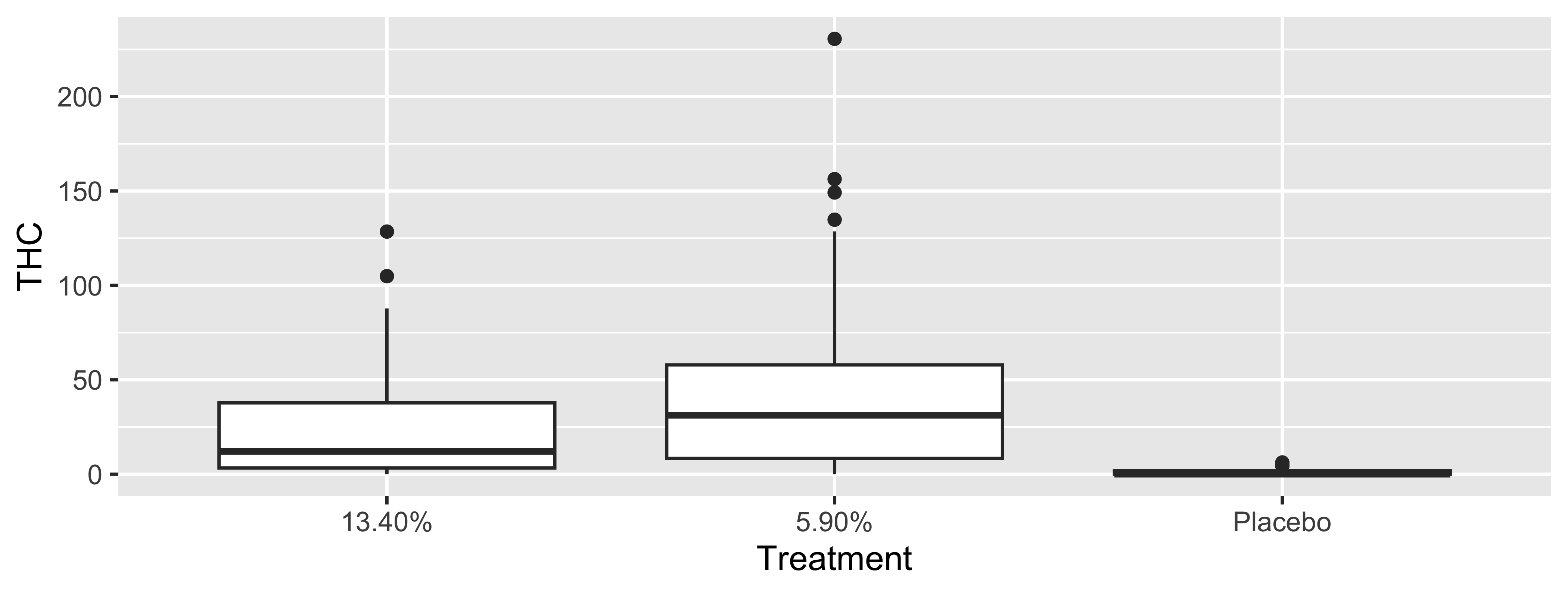

Note: we’ll discuss this specific code soon.

Use `forcats` to manipulate factors

fct_recode - treat as factor; give new labels
fct_relevel - change order of levels

WB_sub <- WB_sub |>
  mutate(Treatment = fct_recode(Treatment, 
                                "5.9% THC (low dose)" = "5.90%",
                                "13.4% THC (high dose)" = "13.40%"),
         Treatment = fct_relevel(Treatment, "Placebo", "5.9% THC (low dose)"))

. . .

(same plotting code as earlier)

WB_sub |> 
  filter(start_time > 0, start_time < 60) |> 
  ggplot(mapping = aes(x = Treatment, y=THC)) +
    geom_boxplot()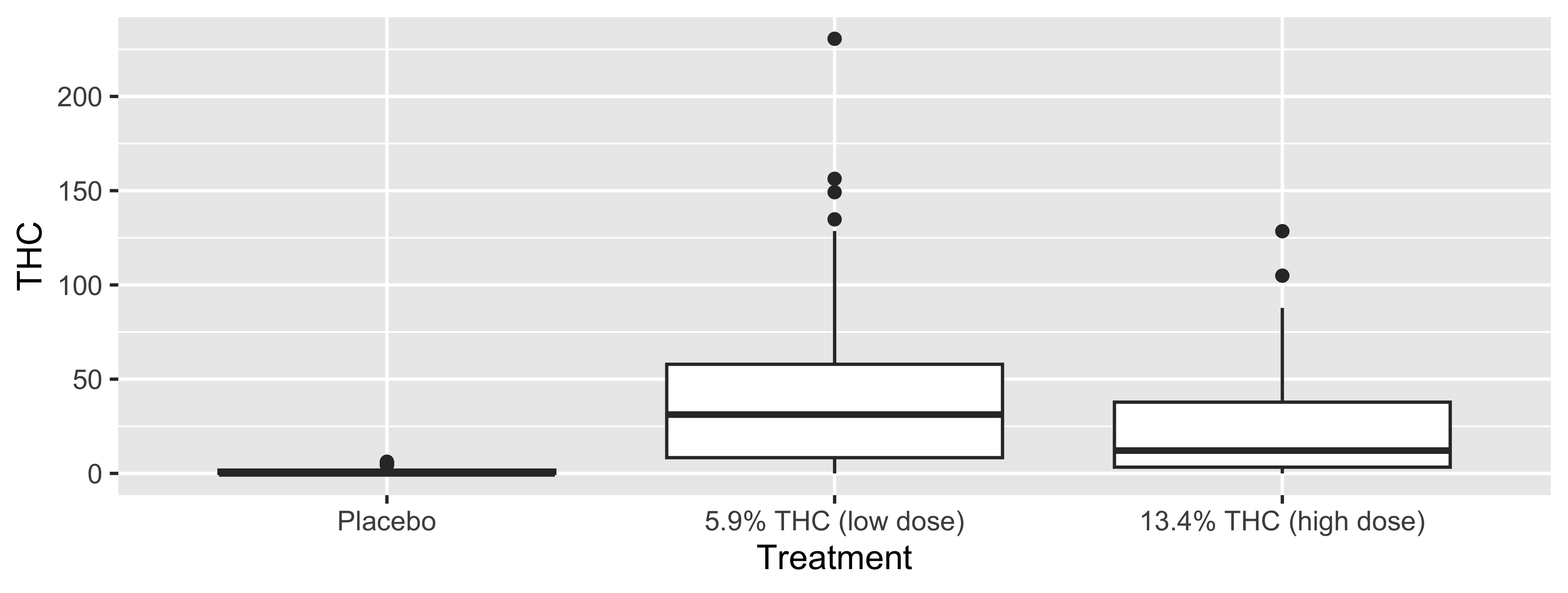

`forcats` functionality

R uses factors to handle categorical variables, variables that have a fixed and known set of possible values. Historically, factors were much easier to work with than character vectors, so many base R functions automatically convert character vectors to factors.
factors are still useful when you have true categorical data, and when you want to override the ordering of character vectors to improve display. The goal of the forcats package is to provide a suite of useful tools that solve common problems with factors.

Source: forcats.tidyverse.org

CS01: Wrangling

Data Cleaning

WB <- WB |> 
  mutate(Treatment = fct_recode(Treatment, 
                                "5.9% THC (low dose)" = "5.90%",
                                "13.4% THC (high dose)" = "13.40%"),
         Treatment = fct_relevel(Treatment, "Placebo", "5.9% THC (low dose)")) |> 
  janitor::clean_names() |>
  rename(thcoh = x11_oh_thc,
         thccooh = thc_cooh,
         thccooh_gluc = thc_cooh_gluc,
         thcv = thc_v)

What is this code accomplishing?

Data Cleaning

WB |> 
  mutate(timepoint = case_when(time_from_start < 0 ~ "pre-smoking",
                               time_from_start > 0 & time_from_start <= 30 ~ "0-30 min",
                               time_from_start > 30 & time_from_start <= 70 ~ "31-70 min",
                               time_from_start > 70 & time_from_start <= 100 ~ "71-100 min",
                               time_from_start > 100 & time_from_start <= 180 ~ "101-180 min",
                               time_from_start > 180 & time_from_start <= 210 ~ "181-210 min",
                               time_from_start > 210 & time_from_start <= 240 ~ "211-240 min",
                               time_from_start > 240 & time_from_start <= 270 ~ "241-270 min",
                               time_from_start > 270 & time_from_start <= 300 ~ "271-300 min",
                               time_from_start > 300 ~ "301+ min"))

# A tibble: 1,525 × 14
   id    treatment    group fluid_type timepoint   cbn   cbd   thc thcoh thccooh
   <chr> <fct>        <chr> <chr>      <chr>     <dbl> <dbl> <dbl> <dbl>   <dbl>
 1 11255 5.9% THC (l… Occa… WB         pre-smok…   0       0   0.5   0       5.7
 2 11255 5.9% THC (l… Occa… WB         0-30 min    2.8     0  32.4   5.4    13.5
 3 11255 5.9% THC (l… Occa… WB         31-70 min   0.6     0   5.1   2.4    11.7
 4 11255 5.9% THC (l… Occa… WB         101-180 …   0       0   3.2   1.8     9.7
 5 11255 5.9% THC (l… Occa… WB         101-180 …   0       0   1.8   1.4     8.7
 6 11255 5.9% THC (l… Occa… WB         211-240 …   0       0   1.2   0       6.7
 7 11255 5.9% THC (l… Occa… WB         271-300 …   0       0   0.9   0       6.8
 8 11255 5.9% THC (l… Occa… WB         301+ min    0       0   0.8   0       6.8
 9 11255 5.9% THC (l… Occa… WB         301+ min    0       0   0.6   0       6.3
10 T0686 5.9% THC (l… Freq… WB         pre-smok…   0       0   0     0       1.9
# ℹ 1,515 more rows
# ℹ 4 more variables: thccooh_gluc <dbl>, cbg <dbl>, thcv <dbl>,
#   time_from_start <dbl>

What is this code accomplishing?

. . .

Note: This code could have been combined with the above…I just wanted to discuss it for simplicity in lecture separately.

CS01 Data Cleaning

We’ve cleaned up the whole blood data. Your lab will guide you to clean up the oral fluid and breath data. (It will be similar, but not the same as this.)

Recap

Understand the basic tenants of dplyr
Describe and utilize the pipe in workflows
Describe and use common verbs (functions)
Understand the documentation for dplyr functions
Understand what factors are an that forcats is a package with functionality for working with them
Describe the wrangling carried out on the CS01 WB dataset

Data Manipulation with dplyr

[ad] EDGE

Q&A

Course Announcements

Suggested Reading

Agenda

Philosophy

Pipes

The pipe in baseR

Where does the name come from?

How does a pipe work?

Data

Whole Blood (WB) Data from THC Study

Variables

Viewing your data

dplyr

A Grammar of Data Manipulation

dplyr rules for functions

Filter rows with filter

filter (single condition)

filter (mutiple conditions)

select` a range of variables

select to keep range + others

select to exclude variables

select can rename columns

“Save” when you make dataset changes

Check before you move on

rename specific columns

mutate to add new variables

Your Turn

group_by + summarize to reduce variables to values

count to group by then count

Your Turn

and arrange to order rows

distinct to filter for unique rows

distinct has a .keep_all parameter

Factors

Factors

Why does it matter?

Use forcats to manipulate factors

forcats functionality

CS01: Wrangling

Data Cleaning

Data Cleaning

CS01 Data Cleaning

Recap

Data Manipulation with `dplyr`

`dplyr`

`dplyr` rules for functions

Filter rows with `filter`

`filter` (single condition)

`filter` (mutiple conditions)

`select` to keep range + others

`select` to exclude variables

`select` can rename columns

`rename` specific columns

`mutate` to add new variables

`group_by` + `summarize` to reduce variables to values

`count` to group by then count

and `arrange` to order rows

`distinct` to filter for unique rows

`distinct` has a `.keep_all` parameter

Use `forcats` to manipulate factors

`forcats` functionality