13-cs02-analysis

Author

Affiliation

Professor Shannon Ellis

UC San Diego
COGS 137 - Fall 2024

Published

November 19, 2024

CS02: Predicting Air Pollution (Analysis)

Q&A

Q: “First, in our CS02, is our prediction US annual average air pollution concentrations based on”“value”“? Is this going to be our outcome, as it was in class?
A: value will be our outcome. In this set of notes, we’ll discuss how to directly answer our question using machine learning.

Q: How do we decide whether to use main effects of interaction effects? Do we have to try both and compare r square values?
A: Well, we only include an interaction term if it actually makes sense for what we’re modelling, if the interaction term’s inclusion makes logical sense - meaning it could impact the relationship between the other predictor and outcome. Without that, it doesn’t make sense to include an interaction term, as the simplest model (no interaction) is preferred overall.

Q: San you redefine the differences between main vs. interaction effects? what are the pros and cons of each?
A: In a main effects model, we’re assuming the relationship between the predictor and outcome does not vary (is not impacted) by the second predictor (different y-intercepts; same slope/rate of change). In an interaction effects model we’re assuming the second predictor does impact the primary predictor and outcomes relationship. (different y-intercepts; different slopes). Con of interaction is that it adds an additional term into the model and is more difficult to interpret. So, you only want to go for an interaction effects model if it truly does a better job capturing the underlying relationships in the data.

Q: I wonder if we will go over logistic regressions, or k-clusters, or any other form of ML algorithms .
A: We’re not going to do logistic regression this quarter, but will introduce ML algorithms in this set of notes!

Course Announcements

Lab07 due Thursday
HW03 due Friday
CS02 due Monday
Final Project - rough draft due Monday

Notes:

Lab06 scores/feedback posted
CS01 scores/feedback posted
- Feedback as issue on repo
- If your score on CS02 is higher than CS01 that score will automatically be used for both CS01 and CS02
Class Thursday will be time to work on CS02

Progress Check-in

❓ Where should you and your group be for CSO2 completion?

. . .

❓ Where should you be at right now for your final project? What should you have done for rough draft on Monday?

Question

With what accuracy can we predict US annual average air pollution concentrations?

Analysis

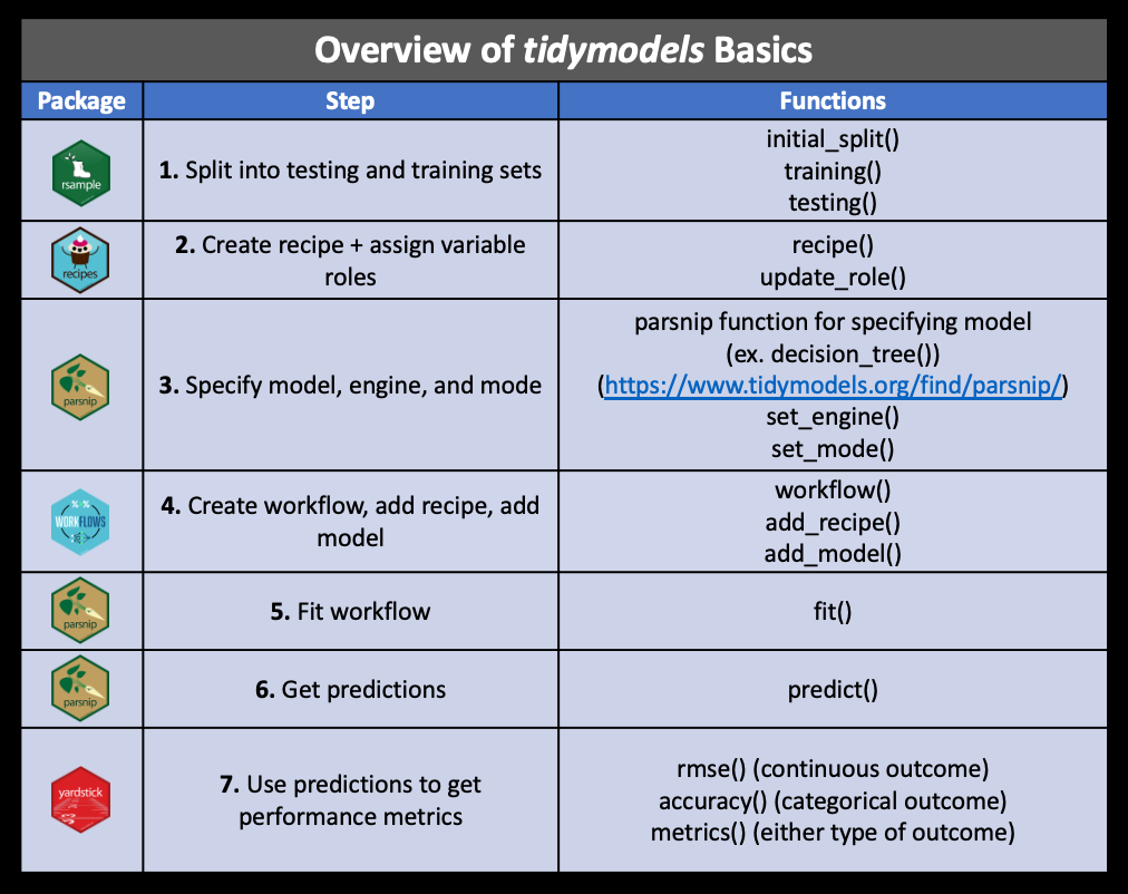
Building our `tidymodels` knowledge:

The Data

pm <- read_csv("OCS_data/data/raw/pm25_data.csv")

# Converting to factors
pm <- pm |>
  mutate(across(c(id, fips, zcta), as.factor))

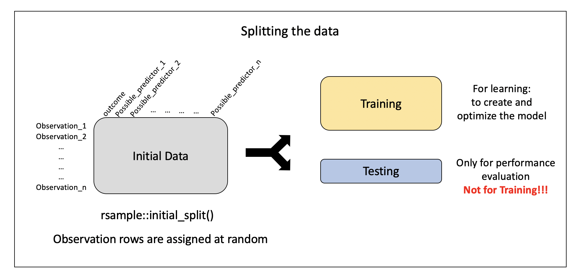
Data Splitting

. . .

Specify the split:

set.seed(1234)
pm_split <- rsample::initial_split(data = pm, prop = 2/3)
pm_split

<Training/Testing/Total>
<584/292/876>

set.seed <- ensures we all get the exact same random split
output displayed: <training data sample number, testing data sample number, original sample number>

More on how people decide what proportions to use for data splitting here

Split the Data

train_pm <- rsample::training(pm_split)
test_pm <- rsample::testing(pm_split)
 
# Scroll through the output!
count(train_pm, state)

# A tibble: 49 × 2
   state                    n
   <chr>                <int>
 1 Alabama                 13
 2 Arizona                 12
 3 Arkansas                 8
 4 California              55
 5 Colorado                10
 6 Connecticut             12
 7 Delaware                 3
 8 District Of Columbia     2
 9 Florida                 22
10 Georgia                 20
# ℹ 39 more rows

❓ What do you observe about the output?

Pre-processing: `recipe()` + `bake()`

Need to:

specify predictors vs. outcome
scale variables
remove redundant variables (feature engineering)

. . .

recipe provides a standardized format for a sequence of steps for pre-processing the data

. . .

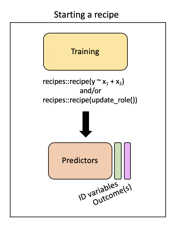
Step 1: Specify variable roles

The simplest approach…

simple_rec <- train_pm |>
  recipes::recipe(value ~ .)

simple_rec

── Recipe ──────────────────────────────────────────────────────────────────────

── Inputs

Number of variables by role

outcome:    1
predictor: 49

. . .

…but we need to specify which column includes ID information

simple_rec <- train_pm |>
  recipes::recipe(value ~ .) |>
  recipes::update_role(id, new_role = "id variable")

simple_rec

── Recipe ──────────────────────────────────────────────────────────────────────

── Inputs

Number of variables by role

outcome:      1
predictor:   48
id variable:  1

. . .

…and which are our predictors and which is our outcome

simple_rec <- recipe(train_pm) |>
    update_role(everything(), new_role = "predictor") |>
    update_role(value, new_role = "outcome") |>
    update_role(id, new_role = "id variable")

simple_rec

── Recipe ──────────────────────────────────────────────────────────────────────

── Inputs

Number of variables by role

outcome:      1
predictor:   48
id variable:  1

❓ Can someone summarize what this code is specifying?

. . .

Summarizing our recipe thus far:

summary(simple_rec)

# A tibble: 50 × 4
   variable type      role        source  
   <chr>    <list>    <chr>       <chr>   
 1 id       <chr [3]> id variable original
 2 value    <chr [2]> outcome     original
 3 fips     <chr [3]> predictor   original
 4 lat      <chr [2]> predictor   original
 5 lon      <chr [2]> predictor   original
 6 state    <chr [3]> predictor   original
 7 county   <chr [3]> predictor   original
 8 city     <chr [3]> predictor   original
 9 CMAQ     <chr [2]> predictor   original
10 zcta     <chr [3]> predictor   original
# ℹ 40 more rows

Step 2: Pre-process with `step*()`

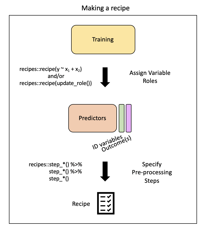
Steps

There are step functions for a variety of purposes:

Imputation – filling in missing values based on the existing data
Transformation – changing all values of a variable in the same way, typically to make it more normal or easier to interpret
Discretization – converting continuous values into discrete or nominal values - binning for example to reduce the number of possible levels (However this is generally not advisable!)
Encoding / Creating Dummy Variables – creating a numeric code for categorical variables (More on one-hot and Dummy Variables encoding)
Data type conversions – which means changing from integer to factor or numeric to date etc.
Interaction term addition to the model – which means that we would be modeling for predictors that would influence the capacity of each other to predict the outcome
Normalization – centering and scaling the data to a similar range of values
Dimensionality Reduction/ Signal Extraction – reducing the space of features or predictors to a smaller set of variables that capture the variation or signal in the original variables (ex. Principal Component Analysis and Independent Component Analysis)
Filtering – filtering options for removing variables (ex. remove variables that are highly correlated to others or remove variables with very little variance and therefore likely little predictive capacity)
Row operations – performing functions on the values within the rows (ex. rearranging, filtering, imputing)
Checking functions – Gut checks to look for missing values, to look at the variable classes etc.

This link and this link show the many options for recipe step functions.

Selecting Variables

There are several ways to select what variables to apply steps to:

Using tidyselect methods: contains(), matches(), starts_with(), ends_with(), everything(), num_range()
Using the type: all_nominal(), all_numeric() , has_type()
Using the role: all_predictors(), all_outcomes(), has_role()
Using the name - use the actual name of the variable/variables of interest

One-hot Encoding

One-hot encoding categorical variables:

simple_rec |>
  step_dummy(state, county, city, zcta, one_hot = TRUE)

── Recipe ──────────────────────────────────────────────────────────────────────

── Inputs

Number of variables by role

outcome:      1
predictor:   48
id variable:  1

── Operations

• Dummy variables from: state, county, city, zcta

❓ Can anyone explain what one-hot encoding does?

. . .

fips includes numeric code for state and county, so it’s another way to specify county
so, we’ll change fips’ role
we get to decide what to call it ("county id")

simple_rec |>
  update_role("fips", new_role = "county id")

── Recipe ──────────────────────────────────────────────────────────────────────

── Inputs

Number of variables by role

outcome:      1
predictor:   47
county id:    1
id variable:  1

. . .

Removing highly correlated variables:

simple_rec |>
  step_corr(all_predictors(), - CMAQ, - aod)

── Recipe ──────────────────────────────────────────────────────────────────────

── Inputs

Number of variables by role

outcome:      1
predictor:   48
id variable:  1

── Operations

• Correlation filter on: all_predictors(), -CMAQ, -aod

specifying to KEEP CMAQ and aod

. . .

Removing variables with non-zero variance:

simple_rec |>
  step_nzv(all_predictors(), - CMAQ, - aod)

── Recipe ──────────────────────────────────────────────────────────────────────

── Inputs

Number of variables by role

outcome:      1
predictor:   48
id variable:  1

── Operations

• Sparse, unbalanced variable filter on: all_predictors(), -CMAQ, -aod

Putting our `recipe` together

simple_rec <- simple_rec |> 
  update_role("fips", new_role = "county id") |>
  step_dummy(state, county, city, zcta, one_hot = TRUE) |>
  step_corr(all_predictors(), - CMAQ, - aod)|>
  step_nzv(all_predictors(), - CMAQ, - aod)
  
simple_rec

── Recipe ──────────────────────────────────────────────────────────────────────

── Inputs

Number of variables by role

outcome:      1
predictor:   47
county id:    1
id variable:  1

── Operations

• Dummy variables from: state, county, city, zcta

• Correlation filter on: all_predictors(), -CMAQ, -aod

• Sparse, unbalanced variable filter on: all_predictors(), -CMAQ, -aod

Note: order of steps matters

Step 3: Running the pre-processing (`prep`)

There are some important arguments to know about:

training - you must supply a training data set to estimate parameters for pre-processing operations (recipe steps) - this may already be included in your recipe - as is the case for us
fresh - if fresh=TRUE, will retrain and estimate parameters for any previous steps that were already prepped if you add more steps to the recipe (default is FALSE)
verbose - if verbose=TRUE, shows the progress as the steps are evaluated and the size of the pre-processed training set (default is FALSE)
retain - if retain=TRUE, then the pre-processed training set will be saved within the recipe (as template). This is good if you are likely to add more steps and do not want to rerun the prep() on the previous steps. However this can make the recipe size large. This is necessary if you want to actually look at the pre-processed data (default is TRUE)

prepped_rec <- prep(simple_rec, 
                    verbose = TRUE, 
                    retain = TRUE )

oper 1 step dummy [training] 
oper 2 step corr [training] 
oper 3 step nzv [training] 
The retained training set is ~ 0.26 Mb  in memory.

names(prepped_rec)

 [1] "var_info"       "term_info"      "steps"          "template"      
 [5] "levels"         "retained"       "requirements"   "tr_info"       
 [9] "orig_lvls"      "last_term_info"

. . .

This output includes a lot of information:

the steps that were run
the original variable info (var_info)
the updated variable info after pre-processing (term_info)
the new levels of the variables
the original levels of the variables (orig_lvls)
info about the training data set size and completeness (tr_info)

Step 4: Extract pre-processed training data using `bake()`

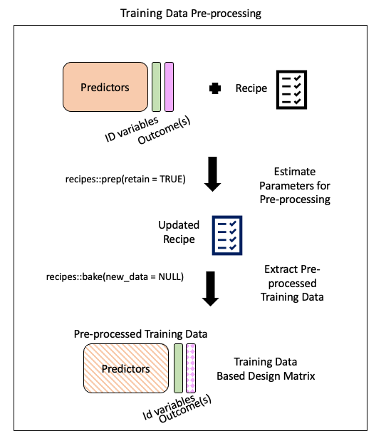
bake(): apply our modeling steps (in this case just pre-processing on the training data) and see what it would do the data

. . .

baked_train <- bake(prepped_rec, new_data = NULL)

glimpse(baked_train)

Rows: 584
Columns: 37
$ id                          <fct> 18003.0004, 55041.0007, 6065.1003, 39009.0…
$ value                       <dbl> 11.699065, 6.956780, 13.289744, 10.742000,…
$ fips                        <fct> 18003, 55041, 6065, 39009, 39061, 24510, 6…
$ lat                         <dbl> 41.09497, 45.56300, 33.94603, 39.44217, 39…
$ lon                         <dbl> -85.10182, -88.80880, -117.40063, -81.9088…
$ CMAQ                        <dbl> 10.383231, 3.411247, 11.404085, 7.971165, …
$ zcta_area                   <dbl> 16696709, 370280916, 41957182, 132383592, …
$ zcta_pop                    <dbl> 21306, 4141, 44001, 1115, 6566, 934, 41192…
$ imp_a500                    <dbl> 28.9783737, 0.0000000, 30.3901384, 0.00000…
$ imp_a15000                  <dbl> 13.0547959, 0.3676404, 23.7457506, 0.33079…
$ county_area                 <dbl> 1702419942, 2626421270, 18664696661, 13043…
$ county_pop                  <dbl> 355329, 9304, 2189641, 64757, 802374, 6209…
$ log_dist_to_prisec          <dbl> 6.621891, 8.415468, 7.419762, 6.344681, 5.…
$ log_pri_length_5000         <dbl> 8.517193, 8.517193, 10.150514, 8.517193, 9…
$ log_pri_length_25000        <dbl> 12.77378, 10.16440, 13.14450, 10.12663, 13…
$ log_prisec_length_500       <dbl> 6.214608, 6.214608, 6.214608, 6.214608, 7.…
$ log_prisec_length_1000      <dbl> 9.240294, 7.600902, 7.600902, 8.793450, 8.…
$ log_prisec_length_5000      <dbl> 11.485093, 9.425537, 10.155961, 10.562382,…
$ log_prisec_length_10000     <dbl> 12.75582, 11.44833, 11.59563, 11.69093, 12…
$ log_nei_2008_pm10_sum_10000 <dbl> 4.91110140, 3.86982666, 4.03184660, 0.0000…
$ log_nei_2008_pm10_sum_15000 <dbl> 5.399131, 3.883689, 5.459257, 0.000000, 6.…
$ log_nei_2008_pm10_sum_25000 <dbl> 5.816047, 3.887264, 6.884537, 3.765635, 6.…
$ popdens_county              <dbl> 208.719947, 3.542463, 117.314577, 49.64834…
$ popdens_zcta                <dbl> 1276.059851, 11.183401, 1048.711994, 8.422…
$ nohs                        <dbl> 4.3, 5.1, 3.7, 4.8, 2.1, 0.0, 2.5, 7.7, 0.…
$ somehs                      <dbl> 6.7, 10.4, 5.9, 11.5, 10.5, 0.0, 4.3, 7.5,…
$ hs                          <dbl> 31.7, 40.3, 17.9, 47.3, 30.0, 0.0, 17.8, 2…
$ somecollege                 <dbl> 27.2, 24.1, 26.3, 20.0, 27.1, 0.0, 26.1, 2…
$ associate                   <dbl> 8.2, 7.4, 8.3, 3.1, 8.5, 71.4, 13.2, 7.6, …
$ bachelor                    <dbl> 15.0, 8.6, 20.2, 9.8, 14.2, 0.0, 23.4, 17.…
$ grad                        <dbl> 6.8, 4.2, 17.7, 3.5, 7.6, 28.6, 12.6, 12.3…
$ pov                         <dbl> 13.500, 18.900, 6.700, 14.400, 12.500, 3.5…
$ hs_orless                   <dbl> 42.7, 55.8, 27.5, 63.6, 42.6, 0.0, 24.6, 3…
$ urc2006                     <dbl> 3, 6, 1, 5, 1, 1, 2, 1, 2, 6, 4, 4, 4, 4, …
$ aod                         <dbl> 54.11111, 31.16667, 83.12500, 33.36364, 50…
$ state_California            <dbl> 0, 0, 1, 0, 0, 0, 1, 1, 0, 0, 0, 1, 0, 0, …
$ city_Not.in.a.city          <dbl> 0, 1, 0, 1, 0, 0, 0, 0, 1, 0, 0, 0, 0, 0, …

new_data = NULL specifies that we’re not (yet) looking at our testing data
We only have 36 variables (33 predictors + 2 id variables + outcome)
categorical variables (state) are gone (one-hot encoding)
state_California remains - only state with nonzero variance (largest # of monitors)

Step 5: Extract pre-processed testing data using `bake()`

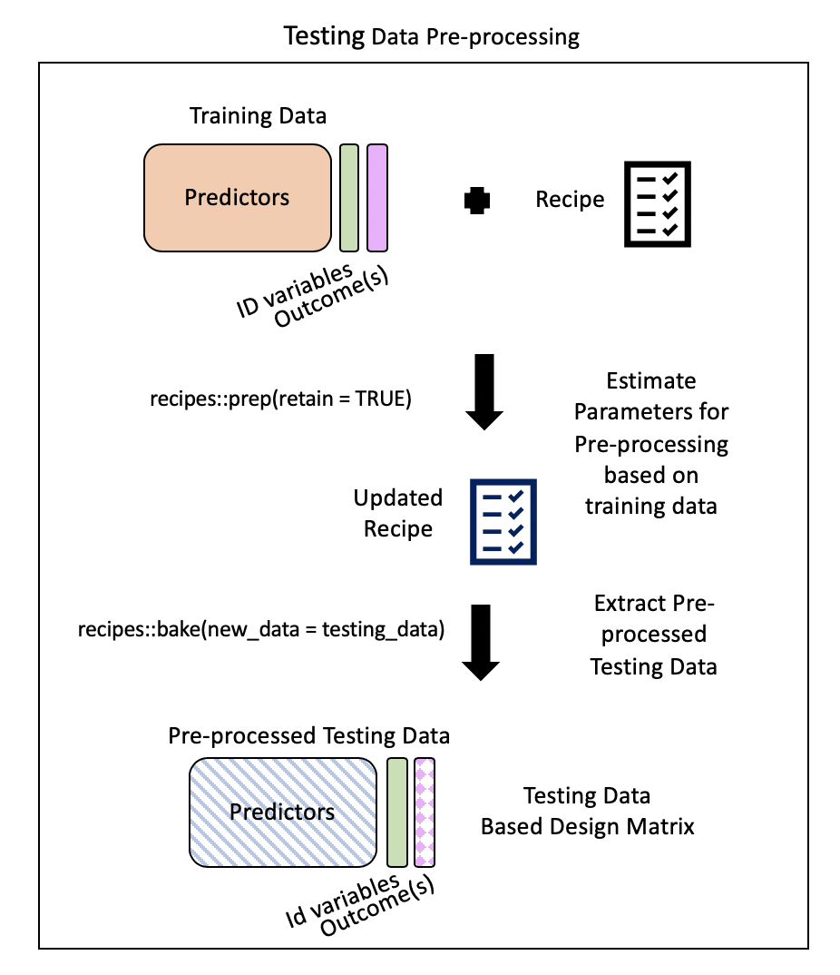
bake() takes a trained recipe and applies the operations to a data set to create a design matrix. For example: it applies the centering to new data sets using these means used to create the recipe. - tidymodels documentation

. . .

Typically, you want to avoid using your testing data…but our data set is not that large and NA values in our testing dataset could cause issues later on.

. . .

baked_test_pm <- recipes::bake(prepped_rec, new_data = test_pm)
glimpse(baked_test_pm)

Rows: 292
Columns: 37
$ id                          <fct> 1033.1002, 1055.001, 1069.0003, 1073.0023,…
$ value                       <dbl> 11.212174, 12.375394, 10.508850, 15.591017…
$ fips                        <fct> 1033, 1055, 1069, 1073, 1073, 1073, 1073, …
$ lat                         <dbl> 34.75878, 33.99375, 31.22636, 33.55306, 33…
$ lon                         <dbl> -87.65056, -85.99107, -85.39077, -86.81500…
$ CMAQ                        <dbl> 9.402679, 9.241744, 9.121892, 10.235612, 1…
$ zcta_area                   <dbl> 16716984, 154069359, 162685124, 26929603, …
$ zcta_pop                    <dbl> 9042, 20045, 30217, 9010, 16140, 3699, 137…
$ imp_a500                    <dbl> 19.17301038, 16.49307958, 19.13927336, 41.…
$ imp_a15000                  <dbl> 5.2472094, 5.1612102, 4.7401296, 17.452484…
$ county_area                 <dbl> 1534877333, 1385618994, 1501737720, 287819…
$ county_pop                  <dbl> 54428, 104430, 101547, 658466, 658466, 194…
$ log_dist_to_prisec          <dbl> 5.760131, 5.261457, 7.112373, 6.600958, 6.…
$ log_pri_length_5000         <dbl> 8.517193, 9.066563, 8.517193, 11.156977, 1…
$ log_pri_length_25000        <dbl> 10.15769, 12.01356, 10.12663, 12.98762, 12…
$ log_prisec_length_500       <dbl> 8.611945, 8.740680, 6.214608, 6.214608, 6.…
$ log_prisec_length_1000      <dbl> 9.735569, 9.627898, 7.600902, 9.075921, 8.…
$ log_prisec_length_5000      <dbl> 11.770407, 11.728889, 12.298627, 12.281645…
$ log_prisec_length_10000     <dbl> 12.840663, 12.768279, 12.994141, 13.278416…
$ log_nei_2008_pm10_sum_10000 <dbl> 6.69187313, 4.43719884, 0.92888890, 8.2097…
$ log_nei_2008_pm10_sum_15000 <dbl> 6.70127741, 4.46267932, 3.67473904, 8.6488…
$ log_nei_2008_pm10_sum_25000 <dbl> 7.148858, 4.678311, 3.744629, 8.858019, 8.…
$ popdens_county              <dbl> 35.460814, 75.367038, 67.619664, 228.77763…
$ popdens_zcta                <dbl> 540.8870404, 130.1037411, 185.7391706, 334…
$ nohs                        <dbl> 7.3, 4.3, 5.8, 7.1, 2.7, 11.1, 9.7, 3.0, 8…
$ somehs                      <dbl> 15.8, 13.3, 11.6, 17.1, 6.6, 11.6, 21.6, 1…
$ hs                          <dbl> 30.6, 27.8, 29.8, 37.2, 30.7, 46.0, 39.3, …
$ somecollege                 <dbl> 20.9, 29.2, 21.4, 23.5, 25.7, 17.2, 21.6, …
$ associate                   <dbl> 7.6, 10.1, 7.9, 7.3, 8.0, 4.1, 5.2, 6.6, 4…
$ bachelor                    <dbl> 12.7, 10.0, 13.7, 5.9, 17.6, 7.1, 2.2, 7.8…
$ grad                        <dbl> 5.1, 5.4, 9.8, 2.0, 8.7, 2.9, 0.4, 4.2, 3.…
$ pov                         <dbl> 19.0, 8.8, 15.6, 25.5, 7.3, 8.1, 13.3, 23.…
$ hs_orless                   <dbl> 53.7, 45.4, 47.2, 61.4, 40.0, 68.7, 70.6, …
$ urc2006                     <dbl> 4, 4, 4, 1, 1, 1, 2, 3, 3, 3, 2, 5, 4, 1, …
$ aod                         <dbl> 36.000000, 43.416667, 33.000000, 39.583333…
$ state_California            <dbl> 0, 0, 0, 0, 0, 0, 0, 0, 0, 0, 0, 0, 0, 0, …
$ city_Not.in.a.city          <dbl> NA, NA, NA, 0, 1, 1, 1, NA, NA, NA, 0, NA,…

. . .

Hmm….lots of NAs now in city_Not.in.a.city

Likely b/c there are cities in our testing dataset that were not in our training dataset…

traincities <- train_pm |> distinct(city)
testcities <- test_pm |> distinct(city)

#get the number of cities that were different
dim(dplyr::setdiff(traincities, testcities))

[1] 381   1

#get the number of cities that overlapped
dim(dplyr::intersect(traincities, testcities))

[1] 55  1

Aside: return to wrangling

A quick return to wrangling…and re-splitting our data

pm <- pm |>
  mutate(city = case_when(city == "Not in a city" ~ "Not in a city",
                          city != "Not in a city" ~ "In a city"))

set.seed(1234) # same seed as before
pm_split <- rsample::initial_split(data = pm, prop = 2/3)
pm_split

<Training/Testing/Total>
<584/292/876>

 train_pm <- rsample::training(pm_split)
 test_pm <- rsample::testing(pm_split)

. . .

And a recipe update…(putting it all together)

novel_rec <- recipe(train_pm) |>
    update_role(everything(), new_role = "predictor") |>
    update_role(value, new_role = "outcome") |>
    update_role(id, new_role = "id variable") |>
    update_role("fips", new_role = "county id") |>
    step_dummy(state, county, city, zcta, one_hot = TRUE) |>
    step_corr(all_numeric()) |>
    step_nzv(all_numeric())

. . .

re-bake()

prepped_rec <- prep(novel_rec, verbose = TRUE, retain = TRUE)

oper 1 step dummy [training] 
oper 2 step corr [training] 
oper 3 step nzv [training] 
The retained training set is ~ 0.27 Mb  in memory.

baked_train <- bake(prepped_rec, new_data = NULL)

. . .

Looking at the output

glimpse(baked_train)

Rows: 584
Columns: 38
$ id                          <fct> 18003.0004, 55041.0007, 6065.1003, 39009.0…
$ value                       <dbl> 11.699065, 6.956780, 13.289744, 10.742000,…
$ fips                        <fct> 18003, 55041, 6065, 39009, 39061, 24510, 6…
$ lat                         <dbl> 41.09497, 45.56300, 33.94603, 39.44217, 39…
$ lon                         <dbl> -85.10182, -88.80880, -117.40063, -81.9088…
$ CMAQ                        <dbl> 10.383231, 3.411247, 11.404085, 7.971165, …
$ zcta_area                   <dbl> 16696709, 370280916, 41957182, 132383592, …
$ zcta_pop                    <dbl> 21306, 4141, 44001, 1115, 6566, 934, 41192…
$ imp_a500                    <dbl> 28.9783737, 0.0000000, 30.3901384, 0.00000…
$ imp_a15000                  <dbl> 13.0547959, 0.3676404, 23.7457506, 0.33079…
$ county_area                 <dbl> 1702419942, 2626421270, 18664696661, 13043…
$ county_pop                  <dbl> 355329, 9304, 2189641, 64757, 802374, 6209…
$ log_dist_to_prisec          <dbl> 6.621891, 8.415468, 7.419762, 6.344681, 5.…
$ log_pri_length_5000         <dbl> 8.517193, 8.517193, 10.150514, 8.517193, 9…
$ log_pri_length_25000        <dbl> 12.77378, 10.16440, 13.14450, 10.12663, 13…
$ log_prisec_length_500       <dbl> 6.214608, 6.214608, 6.214608, 6.214608, 7.…
$ log_prisec_length_1000      <dbl> 9.240294, 7.600902, 7.600902, 8.793450, 8.…
$ log_prisec_length_5000      <dbl> 11.485093, 9.425537, 10.155961, 10.562382,…
$ log_prisec_length_10000     <dbl> 12.75582, 11.44833, 11.59563, 11.69093, 12…
$ log_prisec_length_25000     <dbl> 13.98749, 13.15082, 13.44293, 13.58697, 14…
$ log_nei_2008_pm10_sum_10000 <dbl> 4.91110140, 3.86982666, 4.03184660, 0.0000…
$ log_nei_2008_pm10_sum_15000 <dbl> 5.399131, 3.883689, 5.459257, 0.000000, 6.…
$ log_nei_2008_pm10_sum_25000 <dbl> 5.816047, 3.887264, 6.884537, 3.765635, 6.…
$ popdens_county              <dbl> 208.719947, 3.542463, 117.314577, 49.64834…
$ popdens_zcta                <dbl> 1276.059851, 11.183401, 1048.711994, 8.422…
$ nohs                        <dbl> 4.3, 5.1, 3.7, 4.8, 2.1, 0.0, 2.5, 7.7, 0.…
$ somehs                      <dbl> 6.7, 10.4, 5.9, 11.5, 10.5, 0.0, 4.3, 7.5,…
$ hs                          <dbl> 31.7, 40.3, 17.9, 47.3, 30.0, 0.0, 17.8, 2…
$ somecollege                 <dbl> 27.2, 24.1, 26.3, 20.0, 27.1, 0.0, 26.1, 2…
$ associate                   <dbl> 8.2, 7.4, 8.3, 3.1, 8.5, 71.4, 13.2, 7.6, …
$ bachelor                    <dbl> 15.0, 8.6, 20.2, 9.8, 14.2, 0.0, 23.4, 17.…
$ grad                        <dbl> 6.8, 4.2, 17.7, 3.5, 7.6, 28.6, 12.6, 12.3…
$ pov                         <dbl> 13.500, 18.900, 6.700, 14.400, 12.500, 3.5…
$ hs_orless                   <dbl> 42.7, 55.8, 27.5, 63.6, 42.6, 0.0, 24.6, 3…
$ urc2006                     <dbl> 3, 6, 1, 5, 1, 1, 2, 1, 2, 6, 4, 4, 4, 4, …
$ aod                         <dbl> 54.11111, 31.16667, 83.12500, 33.36364, 50…
$ state_California            <dbl> 0, 0, 1, 0, 0, 0, 1, 1, 0, 0, 0, 1, 0, 0, …
$ city_Not.in.a.city          <dbl> 0, 1, 0, 1, 0, 0, 0, 0, 1, 0, 0, 0, 0, 0, …

. . .

Making sure the NA issue is taken are of:

baked_test_pm <- bake(prepped_rec, new_data = test_pm)

glimpse(baked_test_pm)

Rows: 292
Columns: 38
$ id                          <fct> 1033.1002, 1055.001, 1069.0003, 1073.0023,…
$ value                       <dbl> 11.212174, 12.375394, 10.508850, 15.591017…
$ fips                        <fct> 1033, 1055, 1069, 1073, 1073, 1073, 1073, …
$ lat                         <dbl> 34.75878, 33.99375, 31.22636, 33.55306, 33…
$ lon                         <dbl> -87.65056, -85.99107, -85.39077, -86.81500…
$ CMAQ                        <dbl> 9.402679, 9.241744, 9.121892, 10.235612, 1…
$ zcta_area                   <dbl> 16716984, 154069359, 162685124, 26929603, …
$ zcta_pop                    <dbl> 9042, 20045, 30217, 9010, 16140, 3699, 137…
$ imp_a500                    <dbl> 19.17301038, 16.49307958, 19.13927336, 41.…
$ imp_a15000                  <dbl> 5.2472094, 5.1612102, 4.7401296, 17.452484…
$ county_area                 <dbl> 1534877333, 1385618994, 1501737720, 287819…
$ county_pop                  <dbl> 54428, 104430, 101547, 658466, 658466, 194…
$ log_dist_to_prisec          <dbl> 5.760131, 5.261457, 7.112373, 6.600958, 6.…
$ log_pri_length_5000         <dbl> 8.517193, 9.066563, 8.517193, 11.156977, 1…
$ log_pri_length_25000        <dbl> 10.15769, 12.01356, 10.12663, 12.98762, 12…
$ log_prisec_length_500       <dbl> 8.611945, 8.740680, 6.214608, 6.214608, 6.…
$ log_prisec_length_1000      <dbl> 9.735569, 9.627898, 7.600902, 9.075921, 8.…
$ log_prisec_length_5000      <dbl> 11.770407, 11.728889, 12.298627, 12.281645…
$ log_prisec_length_10000     <dbl> 12.840663, 12.768279, 12.994141, 13.278416…
$ log_prisec_length_25000     <dbl> 13.79973, 13.70026, 13.85550, 14.45221, 13…
$ log_nei_2008_pm10_sum_10000 <dbl> 6.69187313, 4.43719884, 0.92888890, 8.2097…
$ log_nei_2008_pm10_sum_15000 <dbl> 6.70127741, 4.46267932, 3.67473904, 8.6488…
$ log_nei_2008_pm10_sum_25000 <dbl> 7.148858, 4.678311, 3.744629, 8.858019, 8.…
$ popdens_county              <dbl> 35.460814, 75.367038, 67.619664, 228.77763…
$ popdens_zcta                <dbl> 540.8870404, 130.1037411, 185.7391706, 334…
$ nohs                        <dbl> 7.3, 4.3, 5.8, 7.1, 2.7, 11.1, 9.7, 3.0, 8…
$ somehs                      <dbl> 15.8, 13.3, 11.6, 17.1, 6.6, 11.6, 21.6, 1…
$ hs                          <dbl> 30.6, 27.8, 29.8, 37.2, 30.7, 46.0, 39.3, …
$ somecollege                 <dbl> 20.9, 29.2, 21.4, 23.5, 25.7, 17.2, 21.6, …
$ associate                   <dbl> 7.6, 10.1, 7.9, 7.3, 8.0, 4.1, 5.2, 6.6, 4…
$ bachelor                    <dbl> 12.7, 10.0, 13.7, 5.9, 17.6, 7.1, 2.2, 7.8…
$ grad                        <dbl> 5.1, 5.4, 9.8, 2.0, 8.7, 2.9, 0.4, 4.2, 3.…
$ pov                         <dbl> 19.0, 8.8, 15.6, 25.5, 7.3, 8.1, 13.3, 23.…
$ hs_orless                   <dbl> 53.7, 45.4, 47.2, 61.4, 40.0, 68.7, 70.6, …
$ urc2006                     <dbl> 4, 4, 4, 1, 1, 1, 2, 3, 3, 3, 2, 5, 4, 1, …
$ aod                         <dbl> 36.000000, 43.416667, 33.000000, 39.583333…
$ state_California            <dbl> 0, 0, 0, 0, 0, 0, 0, 0, 0, 0, 0, 0, 0, 0, …
$ city_Not.in.a.city          <dbl> 0, 0, 0, 0, 1, 1, 1, 0, 0, 0, 0, 0, 0, 0, …

Specifying our model (`parsnip`)

There are four things we need to define about our model:

The type of model (using specific functions in parsnip like rand_forest(), logistic_reg() etc.)
The package or engine that we will use to implement the type of model selected (using the set_engine() function)
The mode of learning - classification or regression (using the set_mode() function)
Any arguments necessary for the model/package selected (using the set_args()function - for example the mtry = argument for random forest which is the number of variables to be used as options for splitting at each tree node)

Step 1: Specify the model

We’ll start with linear regression, but move to random forest
See here for modeling options in parsnip.

lm_PM_model <- parsnip::linear_reg() |>
  parsnip::set_engine("lm") |>
  set_mode("regression")

lm_PM_model

Linear Regression Model Specification (regression)

Computational engine: lm

Step 2: Fit the model

workflows package allows us to keep track of both our pre-processing steps and our model specification
It also allows us to implement fancier optimizations in an automated way and it can also handle post-processing operations.

PM_wflow <- workflows::workflow() |>
            workflows::add_recipe(novel_rec) |>
            workflows::add_model(lm_PM_model)
PM_wflow

══ Workflow ════════════════════════════════════════════════════════════════════
Preprocessor: Recipe
Model: linear_reg()

── Preprocessor ────────────────────────────────────────────────────────────────
3 Recipe Steps

• step_dummy()
• step_corr()
• step_nzv()

── Model ───────────────────────────────────────────────────────────────────────
Linear Regression Model Specification (regression)

Computational engine: lm

❓ Who can explain the difference between a recipe, baking, and a workflow?

Step 3: Prepare the recipe (estimate the parameters)

PM_wflow_fit <- parsnip::fit(PM_wflow, data = train_pm)
PM_wflow_fit

══ Workflow [trained] ══════════════════════════════════════════════════════════
Preprocessor: Recipe
Model: linear_reg()

── Preprocessor ────────────────────────────────────────────────────────────────
3 Recipe Steps

• step_dummy()
• step_corr()
• step_nzv()

── Model ───────────────────────────────────────────────────────────────────────

Call:
stats::lm(formula = ..y ~ ., data = data)

Coefficients:
                (Intercept)                          lat  
                  2.936e+02                    3.261e-02  
                        lon                         CMAQ  
                  1.586e-02                    2.463e-01  
                  zcta_area                     zcta_pop  
                 -3.433e-10                    1.013e-05  
                   imp_a500                   imp_a15000  
                  5.064e-03                   -3.066e-03  
                county_area                   county_pop  
                 -2.324e-11                   -7.576e-08  
         log_dist_to_prisec          log_pri_length_5000  
                  6.214e-02                   -2.006e-01  
       log_pri_length_25000        log_prisec_length_500  
                 -5.411e-02                    2.204e-01  
     log_prisec_length_1000       log_prisec_length_5000  
                  1.154e-01                    2.374e-01  
    log_prisec_length_10000      log_prisec_length_25000  
                 -3.436e-02                    5.224e-01  
log_nei_2008_pm10_sum_10000  log_nei_2008_pm10_sum_15000  
                  1.829e-01                   -2.355e-02  
log_nei_2008_pm10_sum_25000               popdens_county  
                  2.403e-02                    2.203e-05  
               popdens_zcta                         nohs  
                 -2.132e-06                   -2.983e+00  
                     somehs                           hs  
                 -2.956e+00                   -2.962e+00  
                somecollege                    associate  
                 -2.967e+00                   -2.999e+00  
                   bachelor                         grad  
                 -2.979e+00                   -2.978e+00  
                        pov                    hs_orless  
                  1.859e-03                           NA  
                    urc2006                          aod  
                  2.577e-01                    1.535e-02  
           state_California           city_Not.in.a.city  
                  3.114e+00                   -4.250e-02

Step 4: Assess model fit

wflowoutput <- PM_wflow_fit |> 
  extract_fit_parsnip() |> 
  broom::tidy() 

wflowoutput

# A tibble: 36 × 5
   term         estimate std.error statistic       p.value
   <chr>           <dbl>     <dbl>     <dbl>         <dbl>
 1 (Intercept)  2.94e+ 2  1.18e+ 2     2.49  0.0130       
 2 lat          3.26e- 2  2.28e- 2     1.43  0.153        
 3 lon          1.59e- 2  1.01e- 2     1.58  0.115        
 4 CMAQ         2.46e- 1  3.97e- 2     6.20  0.00000000108
 5 zcta_area   -3.43e-10  1.60e-10    -2.15  0.0320       
 6 zcta_pop     1.01e- 5  5.33e- 6     1.90  0.0578       
 7 imp_a500     5.06e- 3  7.42e- 3     0.683 0.495        
 8 imp_a15000  -3.07e- 3  1.16e- 2    -0.263 0.792        
 9 county_area -2.32e-11  1.97e-11    -1.18  0.238        
10 county_pop  -7.58e- 8  9.29e- 8    -0.815 0.415        
# ℹ 26 more rows

We have fit our model on our training data
We have created a model to predict values of air pollution based on the predictors that we have included

. . .

Understanding what variables are most important in our model…

PM_wflow_fit |> 
  extract_fit_parsnip() |> 
  vip::vip(num_features = 10)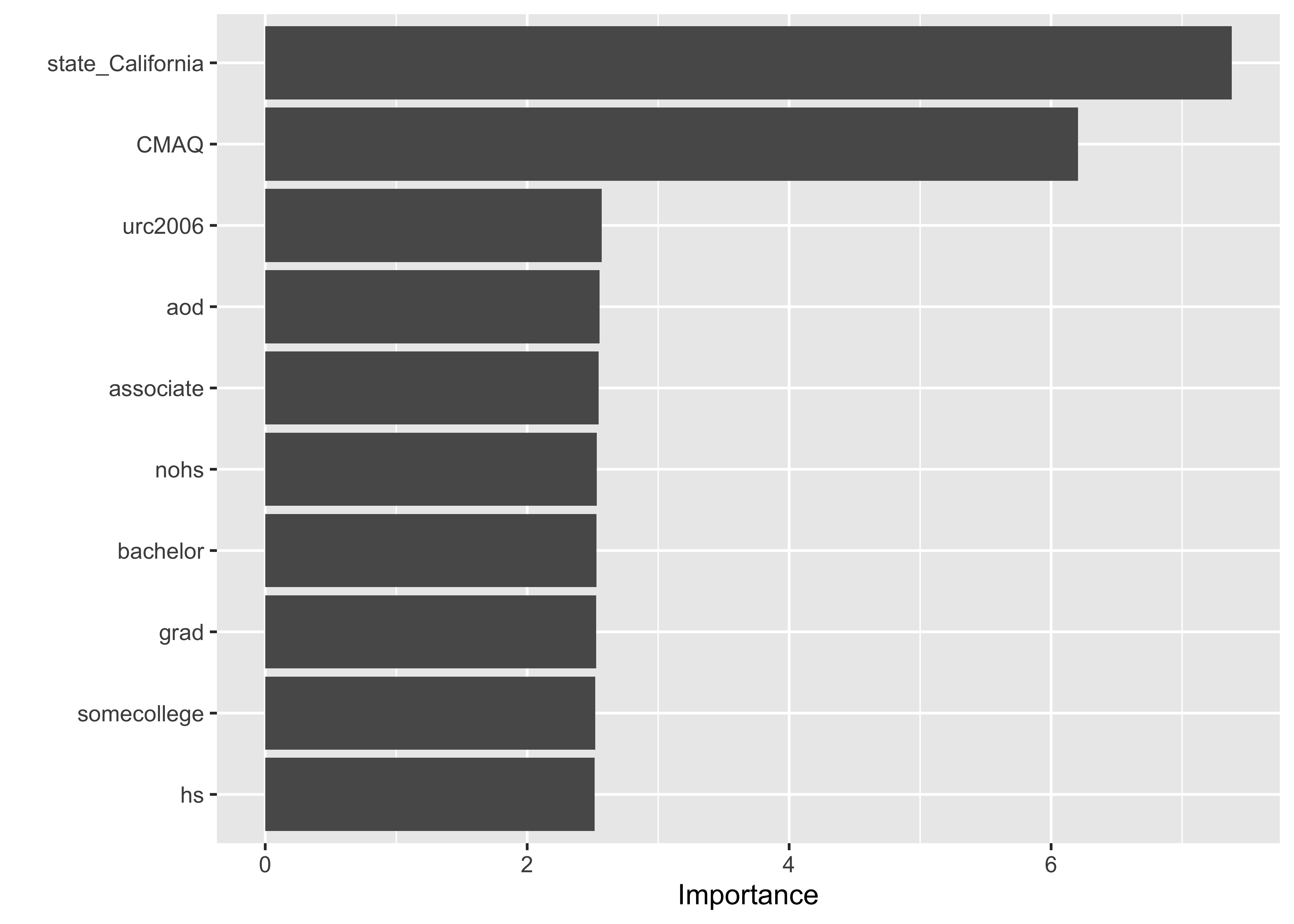

. . .

A closer look at monitors in CA:

baked_train |> 
  mutate(state_California = as.factor(state_California)) |>
  mutate(state_California = recode(state_California, 
                                   "0" = "Not California", 
                                   "1" = "California")) |>
  ggplot(aes(x = state_California, y = value)) + 
  geom_boxplot() +
  geom_jitter(width = .05) + 
  xlab("Location of Monitor")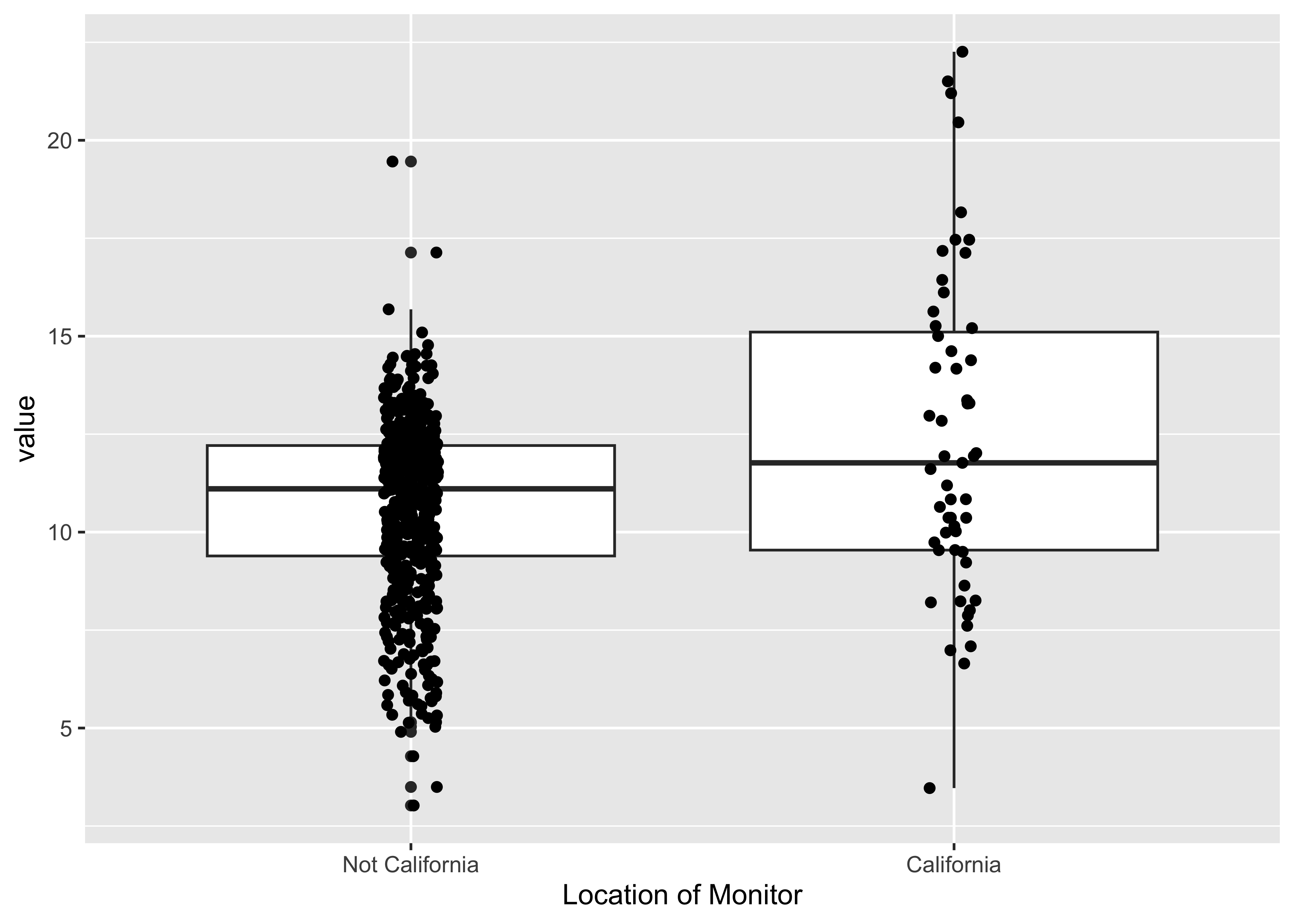

. . .

Remember: machine learning (ML) as an optimization problem that tries to minimize the distance between our predicted outcome \(\hat{Y} = f(X)\) and actual outcome \(Y\) using our features (or predictor variables) \(X\) as input to a function \(f\) that we want to estimate.

\[d(Y - \hat{Y})\]

. . .

Let’s pull out our predicted outcome values \(\hat{Y} = f(X)\) from the models we fit (using different approaches).

wf_fit <- PM_wflow_fit |> 
  extract_fit_parsnip()

wf_fitted_values <- 
  broom::augment(wf_fit[["fit"]], data = baked_train) |> 
  select(value, .fitted:.std.resid)

head(wf_fitted_values)

# A tibble: 6 × 6
  value .fitted   .hat .sigma   .cooksd .std.resid
  <dbl>   <dbl>  <dbl>  <dbl>     <dbl>      <dbl>
1 11.7    12.2  0.0370   2.05 0.0000648     -0.243
2  6.96    9.14 0.0496   2.05 0.00179       -1.09 
3 13.3    12.6  0.0484   2.05 0.000151       0.322
4 10.7    10.4  0.0502   2.05 0.0000504      0.183
5 14.5    11.9  0.0243   2.05 0.00113        1.26 
6 12.2     9.52 0.476    2.04 0.0850         1.81

Visualizing Model Performance

wf_fitted_values |> 
  ggplot(aes(x =  value, y = .fitted)) + 
  geom_point() + 
  xlab("actual outcome values") + 
  ylab("predicted outcome values")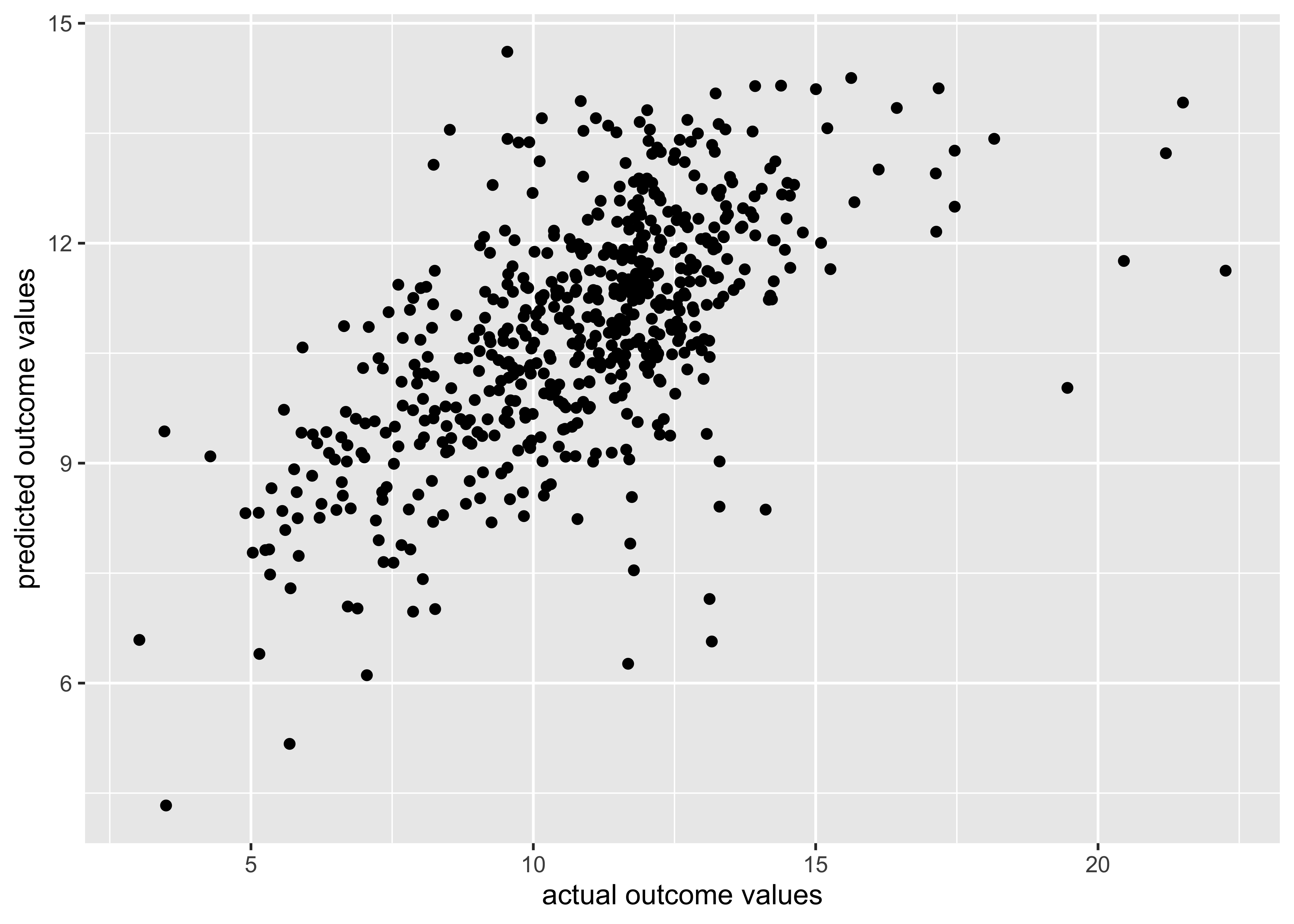

❓ What do you notice about/learn from these results?

Quantifying Model Performance

\[RMSE = \sqrt{\frac{\sum_{i=1}^{n}{(\hat{y_t}- y_t)}^2}{n}}\]

. . .

Can use the yardstick package using the rmse()` function to calculate:

yardstick::metrics(wf_fitted_values,
                   truth = value, estimate = .fitted)

# A tibble: 3 × 3
  .metric .estimator .estimate
  <chr>   <chr>          <dbl>
1 rmse    standard       1.98 
2 rsq     standard       0.392
3 mae     standard       1.47

RMSE isn’t too bad
\(R^2\) suggests model is only explaining 39% of the variance in the data
The MAE value suggests that the average difference between the value predicted and the real value was 1.47 ug/m3. The range of the values was 3-22 in the training data, so this is a relatively small amount

Cross-Validation

Resampling + Re-partitioning:

. . .

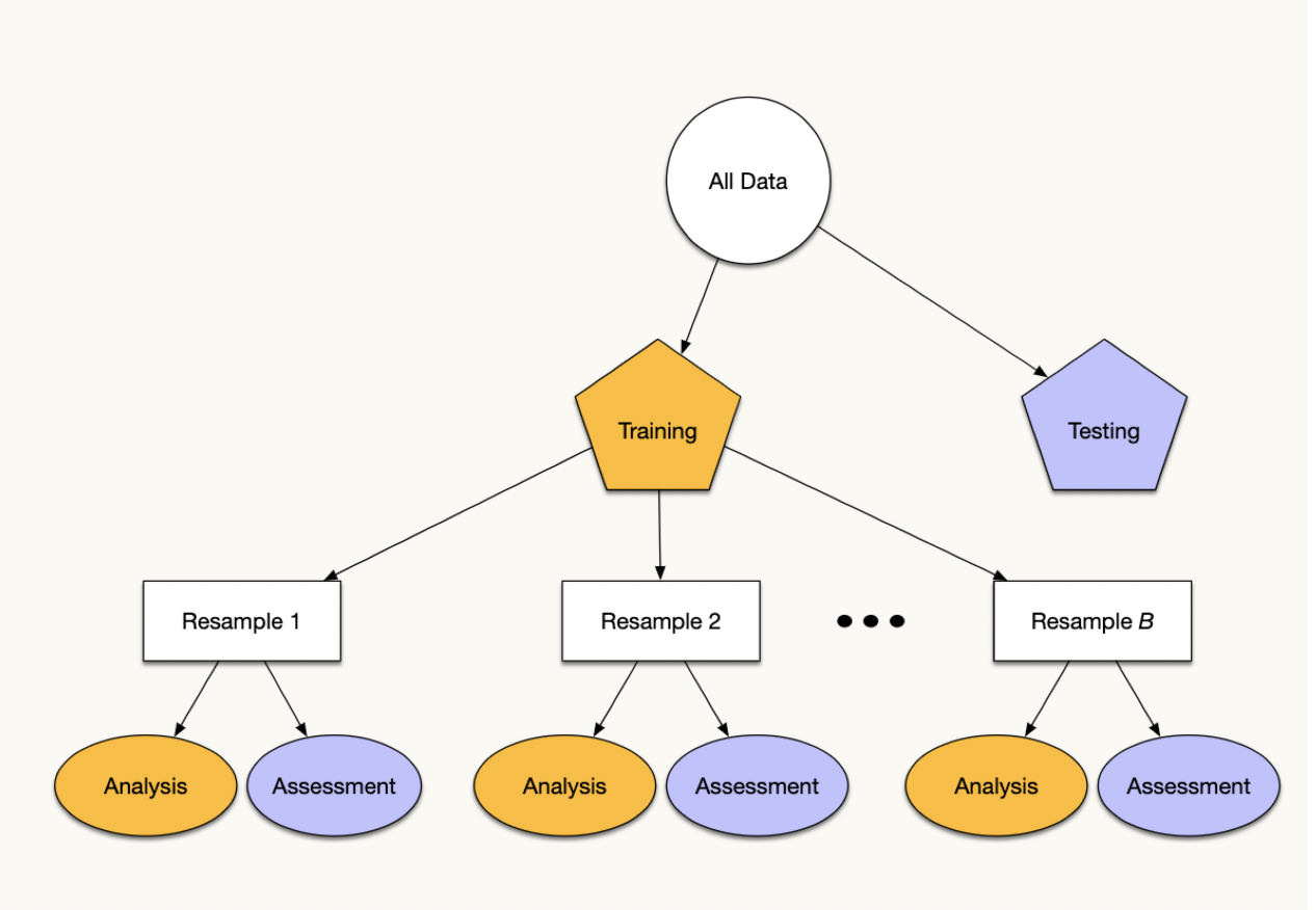
Preparing the data for cross-validation:

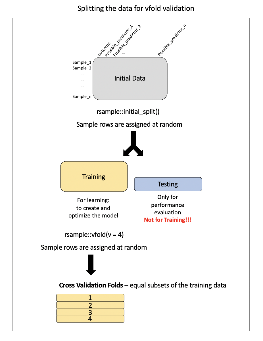
Note: this is called v-fold or k-fold CV

Implementing in `rsample()`

set.seed(1234)
vfold_pm <- rsample::vfold_cv(data = train_pm, v = 4)
vfold_pm

#  4-fold cross-validation 
# A tibble: 4 × 2
  splits            id   
  <list>            <chr>
1 <split [438/146]> Fold1
2 <split [438/146]> Fold2
3 <split [438/146]> Fold3
4 <split [438/146]> Fold4

. . .

pull(vfold_pm, splits)

[[1]]
<Analysis/Assess/Total>
<438/146/584>

[[2]]
<Analysis/Assess/Total>
<438/146/584>

[[3]]
<Analysis/Assess/Total>
<438/146/584>

[[4]]
<Analysis/Assess/Total>
<438/146/584>

. . .

Visualizing this process:

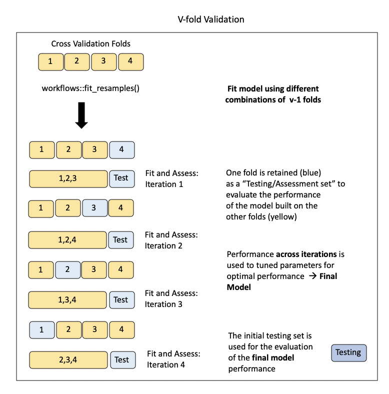
Model Assessment on v-folds

Where this workflow thing really shines…

resample_fit <- tune::fit_resamples(PM_wflow, vfold_pm)

. . .

Gives us a sense of the RMSE across the four folds:

tune::show_best(resample_fit, metric = "rmse")

# A tibble: 1 × 6
  .metric .estimator  mean     n std_err .config             
  <chr>   <chr>      <dbl> <int>   <dbl> <chr>               
1 rmse    standard    2.12     4  0.0444 Preprocessor1_Model1

A different model?

Random Forest

Fitting a different model…is based on a decision tree:

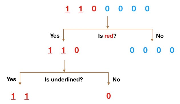
[source]

But not just one tree…

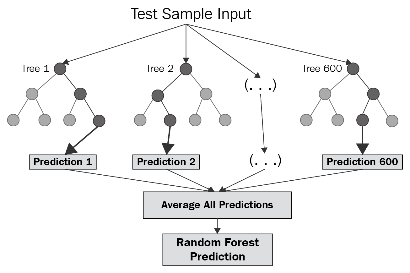
But…in the case of random forest:

multiple decision trees are created (hence: forest),
each tree is built using a random subset of the training data (with replacement) (hence: random)
helps to keep the algorithm from overfitting the data
The mean of the predictions from each of the trees is used in the final output.

Visualizing a RF

Updating our `recipe()`

RF_rec <- recipe(train_pm) |>
    update_role(everything(), new_role = "predictor")|>
    update_role(value, new_role = "outcome")|>
    update_role(id, new_role = "id variable") |>
    update_role("fips", new_role = "county id") |>
    step_novel("state") |>
    step_string2factor("state", "county", "city") |>
    step_rm("county") |>
    step_rm("zcta") |>
    step_corr(all_numeric())|>
    step_nzv(all_numeric())

can use our categorical data as is (no dummy coding)
step_novel()necessary here for the state variable to get all cross validation folds to work, (b/c there will be different levels included in each fold test and training sets. The new levels for some of the test sets would otherwise result in an error.; “step_novel creates a specification of a recipe step that will assign a previously unseen factor level to a new value.”

Model Specification

Model parameters:

mtry - The number of predictor variables (or features) that will be randomly sampled at each split when creating the tree models. The default number for regression analyses is the number of predictors divided by 3.
min_n - The minimum number of data points in a node that are required for the node to be split further.
trees - the number of trees in the ensemble

. . .

# install.packages("randomForest")
RF_PM_model <- parsnip::rand_forest(mtry = 10, min_n = 3) |> 
  set_engine("randomForest") |>
  set_mode("regression")

RF_PM_model

Random Forest Model Specification (regression)

Main Arguments:
  mtry = 10
  min_n = 3

Computational engine: randomForest

Workflow

RF_wflow <- workflows::workflow() |>
  workflows::add_recipe(RF_rec) |>
  workflows::add_model(RF_PM_model)

RF_wflow

══ Workflow ════════════════════════════════════════════════════════════════════
Preprocessor: Recipe
Model: rand_forest()

── Preprocessor ────────────────────────────────────────────────────────────────
6 Recipe Steps

• step_novel()
• step_string2factor()
• step_rm()
• step_rm()
• step_corr()
• step_nzv()

── Model ───────────────────────────────────────────────────────────────────────
Random Forest Model Specification (regression)

Main Arguments:
  mtry = 10
  min_n = 3

Computational engine: randomForest

Fit the Data

RF_wflow_fit <- parsnip::fit(RF_wflow, data = train_pm)

RF_wflow_fit

══ Workflow [trained] ══════════════════════════════════════════════════════════
Preprocessor: Recipe
Model: rand_forest()

── Preprocessor ────────────────────────────────────────────────────────────────
6 Recipe Steps

• step_novel()
• step_string2factor()
• step_rm()
• step_rm()
• step_corr()
• step_nzv()

── Model ───────────────────────────────────────────────────────────────────────

Call:
 randomForest(x = maybe_data_frame(x), y = y, mtry = min_cols(~10,      x), nodesize = min_rows(~3, x)) 
               Type of random forest: regression
                     Number of trees: 500
No. of variables tried at each split: 10

          Mean of squared residuals: 2.633639
                    % Var explained: 59.29

Assess Feature Importance

RF_wflow_fit |> 
  extract_fit_parsnip() |> 
  vip::vip(num_features = 10)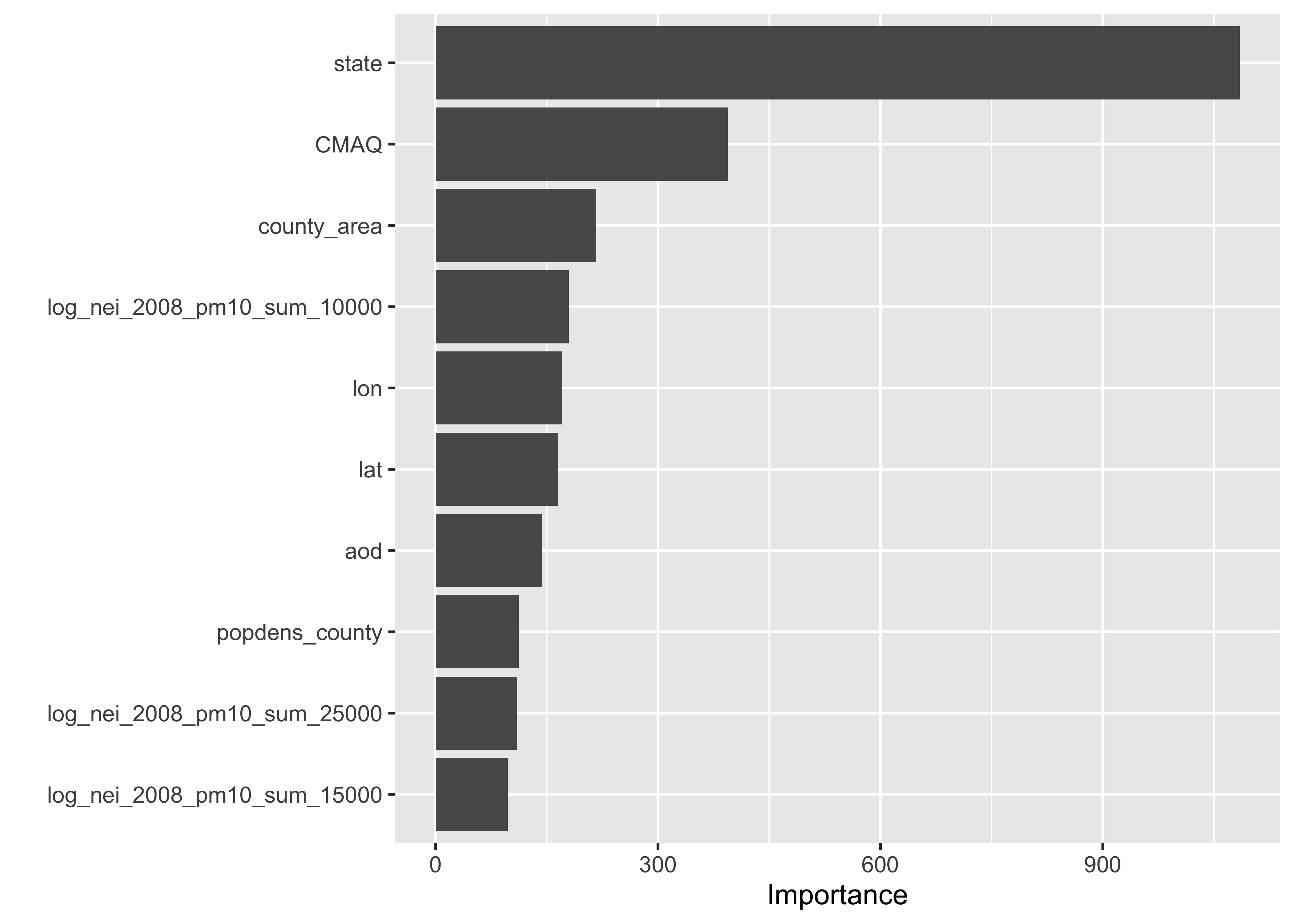

❓ What’s your interpretation of these results?

Assess Model Performance

set.seed(456)
resample_RF_fit <- tune::fit_resamples(RF_wflow, vfold_pm)
collect_metrics(resample_RF_fit)

# A tibble: 2 × 6
  .metric .estimator  mean     n std_err .config             
  <chr>   <chr>      <dbl> <int>   <dbl> <chr>               
1 rmse    standard   1.67      4  0.101  Preprocessor1_Model1
2 rsq     standard   0.591     4  0.0514 Preprocessor1_Model1

. . .

For comparison:

collect_metrics(resample_fit)

# A tibble: 2 × 6
  .metric .estimator  mean     n std_err .config             
  <chr>   <chr>      <dbl> <int>   <dbl> <chr>               
1 rmse    standard   2.12      4  0.0444 Preprocessor1_Model1
2 rsq     standard   0.307     4  0.0263 Preprocessor1_Model1

❓ Thoughts on which model better achieves our goal?

Model Tuning

Hyperparameters are often things that we need to specify about a model. Instead of arbitrarily specifying this, we can try to determine the best option for model performance by a process called tuning.

. . .

Rather than specifying values, we can use tune():

tune_RF_model <- rand_forest(mtry = tune(), min_n = tune()) |>
  set_engine("randomForest") |>
  set_mode("regression")
    
tune_RF_model

Random Forest Model Specification (regression)

Main Arguments:
  mtry = tune()
  min_n = tune()

Computational engine: randomForest

. . .

Create Workflow:

RF_tune_wflow <- workflows::workflow() |>
  workflows::add_recipe(RF_rec) |>
  workflows::add_model(tune_RF_model)

RF_tune_wflow

══ Workflow ════════════════════════════════════════════════════════════════════
Preprocessor: Recipe
Model: rand_forest()

── Preprocessor ────────────────────────────────────────────────────────────────
6 Recipe Steps

• step_novel()
• step_string2factor()
• step_rm()
• step_rm()
• step_corr()
• step_nzv()

── Model ───────────────────────────────────────────────────────────────────────
Random Forest Model Specification (regression)

Main Arguments:
  mtry = tune()
  min_n = tune()

Computational engine: randomForest

Detect how many cores you have access to:

n_cores <- parallel::detectCores()
n_cores

[1] 10

. . .

This code will take some time to run:

# install.packages("doParallel")
doParallel::registerDoParallel(cores = n_cores)

set.seed(123)
tune_RF_results <- tune_grid(object = RF_tune_wflow, resamples = vfold_pm, grid = 20)
tune_RF_results

# Tuning results
# 4-fold cross-validation 
# A tibble: 4 × 4
  splits            id    .metrics          .notes          
  <list>            <chr> <list>            <list>          
1 <split [438/146]> Fold1 <tibble [40 × 6]> <tibble [0 × 3]>
2 <split [438/146]> Fold2 <tibble [40 × 6]> <tibble [0 × 3]>
3 <split [438/146]> Fold3 <tibble [40 × 6]> <tibble [1 × 3]>
4 <split [438/146]> Fold4 <tibble [40 × 6]> <tibble [0 × 3]>

There were issues with some computations:

  - Warning(s) x1: 36 columns were requested but there were 35 predictors in the dat...

Run `show_notes(.Last.tune.result)` for more information.

Check Metrics:

tune_RF_results |>
  collect_metrics()

# A tibble: 40 × 8
    mtry min_n .metric .estimator  mean     n std_err .config              
   <int> <int> <chr>   <chr>      <dbl> <int>   <dbl> <chr>                
 1    12    33 rmse    standard   1.72      4  0.0866 Preprocessor1_Model01
 2    12    33 rsq     standard   0.562     4  0.0466 Preprocessor1_Model01
 3    27    35 rmse    standard   1.69      4  0.102  Preprocessor1_Model02
 4    27    35 rsq     standard   0.563     4  0.0511 Preprocessor1_Model02
 5    22    40 rmse    standard   1.71      4  0.106  Preprocessor1_Model03
 6    22    40 rsq     standard   0.556     4  0.0543 Preprocessor1_Model03
 7     1    27 rmse    standard   2.03      4  0.0501 Preprocessor1_Model04
 8     1    27 rsq     standard   0.440     4  0.0245 Preprocessor1_Model04
 9     6    32 rmse    standard   1.77      4  0.0756 Preprocessor1_Model05
10     6    32 rsq     standard   0.552     4  0.0435 Preprocessor1_Model05
# ℹ 30 more rows

. . .

show_best(tune_RF_results, metric = "rmse", n = 1)

# A tibble: 1 × 8
   mtry min_n .metric .estimator  mean     n std_err .config              
  <int> <int> <chr>   <chr>      <dbl> <int>   <dbl> <chr>                
1    32    11 rmse    standard    1.65     4   0.113 Preprocessor1_Model10

Final Model Evaluation

tuned_RF_values<- select_best(tune_RF_results, "rmse")
tuned_RF_values

# A tibble: 1 × 3
   mtry min_n .config              
  <int> <int> <chr>                
1    32    11 Preprocessor1_Model10

. . .

The testing data!

# specify best combination from tune in workflow
RF_tuned_wflow <-RF_tune_wflow |>
  tune::finalize_workflow(tuned_RF_values)

# fit model with those parameters on train AND test
overallfit <- RF_wflow |>
  tune::last_fit(pm_split)

collect_metrics(overallfit)

# A tibble: 2 × 4
  .metric .estimator .estimate .config             
  <chr>   <chr>          <dbl> <chr>               
1 rmse    standard       1.72  Preprocessor1_Model1
2 rsq     standard       0.608 Preprocessor1_Model1

Results are similar to what we saw in training (RMSE: 1.65)

. . .

Getting the predictions for the test data:

test_predictions <- collect_predictions(overallfit)

Visualizing our results

A map of the US

Packages needed:

sf - the simple features package helps to convert geographical coordinates into geometry variables which are useful for making 2D plots
maps - this package contains geographical outlines and plotting functions to create plots with maps
rnaturalearth- this allows for easy interaction with map data from Natural Earth which is a public domain map dataset

library(sf)
library(maps)
library(rnaturalearth)

Outline of the US

world <- ne_countries(scale = "medium", returnclass = "sf")
glimpse(world)

Rows: 241
Columns: 64
$ scalerank  <int> 3, 1, 1, 1, 1, 3, 3, 1, 1, 1, 3, 1, 5, 3, 1, 1, 1, 1, 1, 1,…
$ featurecla <chr> "Admin-0 country", "Admin-0 country", "Admin-0 country", "A…
$ labelrank  <dbl> 5, 3, 3, 6, 6, 6, 6, 4, 2, 6, 4, 4, 5, 6, 6, 2, 4, 5, 6, 2,…
$ sovereignt <chr> "Netherlands", "Afghanistan", "Angola", "United Kingdom", "…
$ sov_a3     <chr> "NL1", "AFG", "AGO", "GB1", "ALB", "FI1", "AND", "ARE", "AR…
$ adm0_dif   <dbl> 1, 0, 0, 1, 0, 1, 0, 0, 0, 0, 1, 0, 1, 1, 0, 1, 0, 0, 0, 0,…
$ level      <dbl> 2, 2, 2, 2, 2, 2, 2, 2, 2, 2, 2, 2, 2, 2, 2, 2, 2, 2, 2, 2,…
$ type       <chr> "Country", "Sovereign country", "Sovereign country", "Depen…
$ admin      <chr> "Aruba", "Afghanistan", "Angola", "Anguilla", "Albania", "A…
$ adm0_a3    <chr> "ABW", "AFG", "AGO", "AIA", "ALB", "ALD", "AND", "ARE", "AR…
$ geou_dif   <dbl> 0, 0, 0, 0, 0, 0, 0, 0, 0, 0, 0, 0, 0, 0, 0, 0, 0, 0, 0, 0,…
$ geounit    <chr> "Aruba", "Afghanistan", "Angola", "Anguilla", "Albania", "A…
$ gu_a3      <chr> "ABW", "AFG", "AGO", "AIA", "ALB", "ALD", "AND", "ARE", "AR…
$ su_dif     <dbl> 0, 0, 0, 0, 0, 0, 0, 0, 0, 0, 0, 0, 0, 0, 0, 0, 0, 0, 0, 0,…
$ subunit    <chr> "Aruba", "Afghanistan", "Angola", "Anguilla", "Albania", "A…
$ su_a3      <chr> "ABW", "AFG", "AGO", "AIA", "ALB", "ALD", "AND", "ARE", "AR…
$ brk_diff   <dbl> 0, 0, 0, 0, 0, 0, 0, 0, 0, 0, 0, 0, 0, 0, 0, 0, 0, 0, 0, 0,…
$ name       <chr> "Aruba", "Afghanistan", "Angola", "Anguilla", "Albania", "A…
$ name_long  <chr> "Aruba", "Afghanistan", "Angola", "Anguilla", "Albania", "A…
$ brk_a3     <chr> "ABW", "AFG", "AGO", "AIA", "ALB", "ALD", "AND", "ARE", "AR…
$ brk_name   <chr> "Aruba", "Afghanistan", "Angola", "Anguilla", "Albania", "A…
$ brk_group  <chr> NA, NA, NA, NA, NA, NA, NA, NA, NA, NA, NA, NA, NA, NA, NA,…
$ abbrev     <chr> "Aruba", "Afg.", "Ang.", "Ang.", "Alb.", "Aland", "And.", "…
$ postal     <chr> "AW", "AF", "AO", "AI", "AL", "AI", "AND", "AE", "AR", "ARM…
$ formal_en  <chr> "Aruba", "Islamic State of Afghanistan", "People's Republic…
$ formal_fr  <chr> NA, NA, NA, NA, NA, NA, NA, NA, NA, NA, NA, NA, NA, NA, NA,…
$ note_adm0  <chr> "Neth.", NA, NA, "U.K.", NA, "Fin.", NA, NA, NA, NA, "U.S.A…
$ note_brk   <chr> NA, NA, NA, NA, NA, NA, NA, NA, NA, NA, NA, "Multiple claim…
$ name_sort  <chr> "Aruba", "Afghanistan", "Angola", "Anguilla", "Albania", "A…
$ name_alt   <chr> NA, NA, NA, NA, NA, NA, NA, NA, NA, NA, NA, NA, NA, NA, NA,…
$ mapcolor7  <dbl> 4, 5, 3, 6, 1, 4, 1, 2, 3, 3, 4, 4, 1, 7, 2, 1, 3, 1, 2, 3,…
$ mapcolor8  <dbl> 2, 6, 2, 6, 4, 1, 4, 1, 1, 1, 5, 5, 2, 5, 2, 2, 1, 6, 2, 2,…
$ mapcolor9  <dbl> 2, 8, 6, 6, 1, 4, 1, 3, 3, 2, 1, 1, 2, 9, 5, 2, 3, 5, 5, 1,…
$ mapcolor13 <dbl> 9, 7, 1, 3, 6, 6, 8, 3, 13, 10, 1, NA, 7, 11, 5, 7, 4, 8, 8…
$ pop_est    <dbl> 103065, 28400000, 12799293, 14436, 3639453, 27153, 83888, 4…
$ gdp_md_est <dbl> 2258.0, 22270.0, 110300.0, 108.9, 21810.0, 1563.0, 3660.0, …
$ pop_year   <dbl> NA, NA, NA, NA, NA, NA, NA, NA, NA, NA, NA, NA, NA, NA, NA,…
$ lastcensus <dbl> 2010, 1979, 1970, NA, 2001, NA, 1989, 2010, 2010, 2001, 201…
$ gdp_year   <dbl> NA, NA, NA, NA, NA, NA, NA, NA, NA, NA, NA, NA, NA, NA, NA,…
$ economy    <chr> "6. Developing region", "7. Least developed region", "7. Le…
$ income_grp <chr> "2. High income: nonOECD", "5. Low income", "3. Upper middl…
$ wikipedia  <dbl> NA, NA, NA, NA, NA, NA, NA, NA, NA, NA, NA, NA, NA, NA, NA,…
$ fips_10    <chr> NA, NA, NA, NA, NA, NA, NA, NA, NA, NA, NA, NA, NA, NA, NA,…
$ iso_a2     <chr> "AW", "AF", "AO", "AI", "AL", "AX", "AD", "AE", "AR", "AM",…
$ iso_a3     <chr> "ABW", "AFG", "AGO", "AIA", "ALB", "ALA", "AND", "ARE", "AR…
$ iso_n3     <chr> "533", "004", "024", "660", "008", "248", "020", "784", "03…
$ un_a3      <chr> "533", "004", "024", "660", "008", "248", "020", "784", "03…
$ wb_a2      <chr> "AW", "AF", "AO", NA, "AL", NA, "AD", "AE", "AR", "AM", "AS…
$ wb_a3      <chr> "ABW", "AFG", "AGO", NA, "ALB", NA, "ADO", "ARE", "ARG", "A…
$ woe_id     <dbl> NA, NA, NA, NA, NA, NA, NA, NA, NA, NA, NA, NA, NA, NA, NA,…
$ adm0_a3_is <chr> "ABW", "AFG", "AGO", "AIA", "ALB", "ALA", "AND", "ARE", "AR…
$ adm0_a3_us <chr> "ABW", "AFG", "AGO", "AIA", "ALB", "ALD", "AND", "ARE", "AR…
$ adm0_a3_un <dbl> NA, NA, NA, NA, NA, NA, NA, NA, NA, NA, NA, NA, NA, NA, NA,…
$ adm0_a3_wb <dbl> NA, NA, NA, NA, NA, NA, NA, NA, NA, NA, NA, NA, NA, NA, NA,…
$ continent  <chr> "North America", "Asia", "Africa", "North America", "Europe…
$ region_un  <chr> "Americas", "Asia", "Africa", "Americas", "Europe", "Europe…
$ subregion  <chr> "Caribbean", "Southern Asia", "Middle Africa", "Caribbean",…
$ region_wb  <chr> "Latin America & Caribbean", "South Asia", "Sub-Saharan Afr…
$ name_len   <dbl> 5, 11, 6, 8, 7, 5, 7, 20, 9, 7, 14, 10, 23, 22, 17, 9, 7, 1…
$ long_len   <dbl> 5, 11, 6, 8, 7, 13, 7, 20, 9, 7, 14, 10, 27, 35, 19, 9, 7, …
$ abbrev_len <dbl> 5, 4, 4, 4, 4, 5, 4, 6, 4, 4, 9, 4, 7, 10, 6, 4, 5, 4, 4, 5…
$ tiny       <dbl> 4, NA, NA, NA, NA, 5, 5, NA, NA, NA, 3, NA, NA, 2, 4, NA, N…
$ homepart   <dbl> NA, 1, 1, NA, 1, NA, 1, 1, 1, 1, NA, 1, NA, NA, 1, 1, 1, 1,…
$ geometry   <MULTIPOLYGON [°]> MULTIPOLYGON (((-69.89912 1..., MULTIPOLYGON (…

World map:

ggplot(data = world) +
    geom_sf()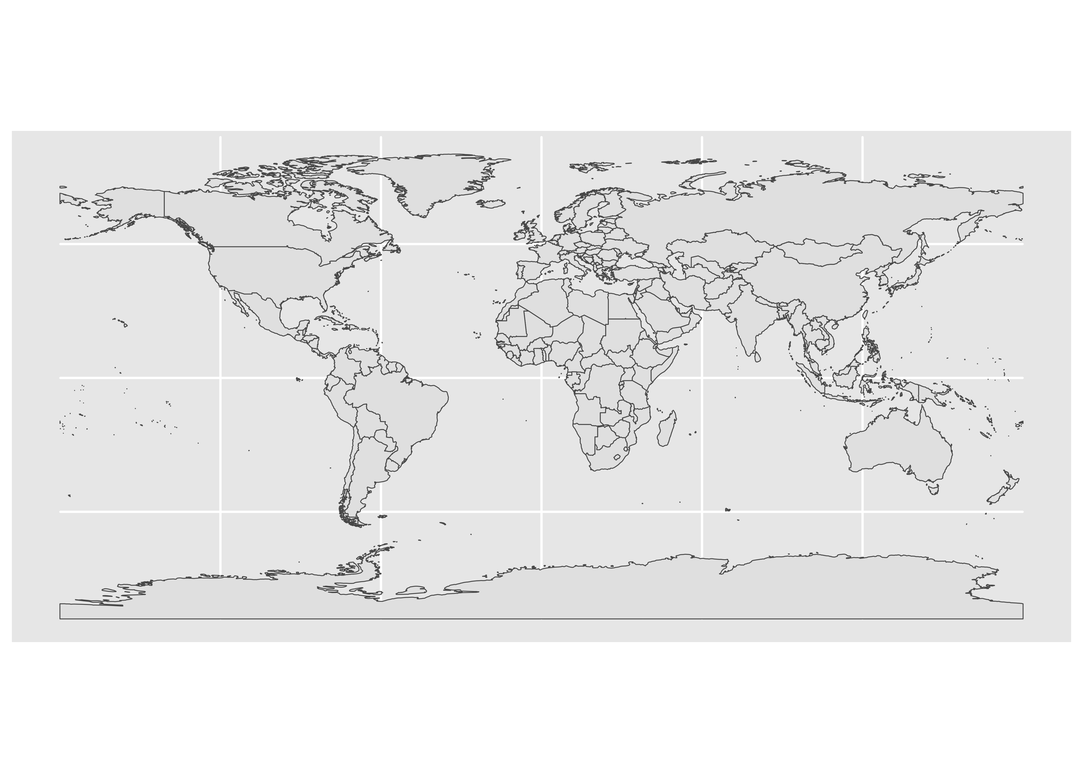

Just the US

According to this link, these are the latitude and longitude bounds of the continental US:

top = 49.3457868 # north lat
left = -124.7844079 # west long
right = -66.9513812 # east long
bottom = 24.7433195 # south lat

Just the US

ggplot(data = world) +
    geom_sf() +
    coord_sf(xlim = c(-125, -66), ylim = c(24.5, 50), 
             expand = FALSE)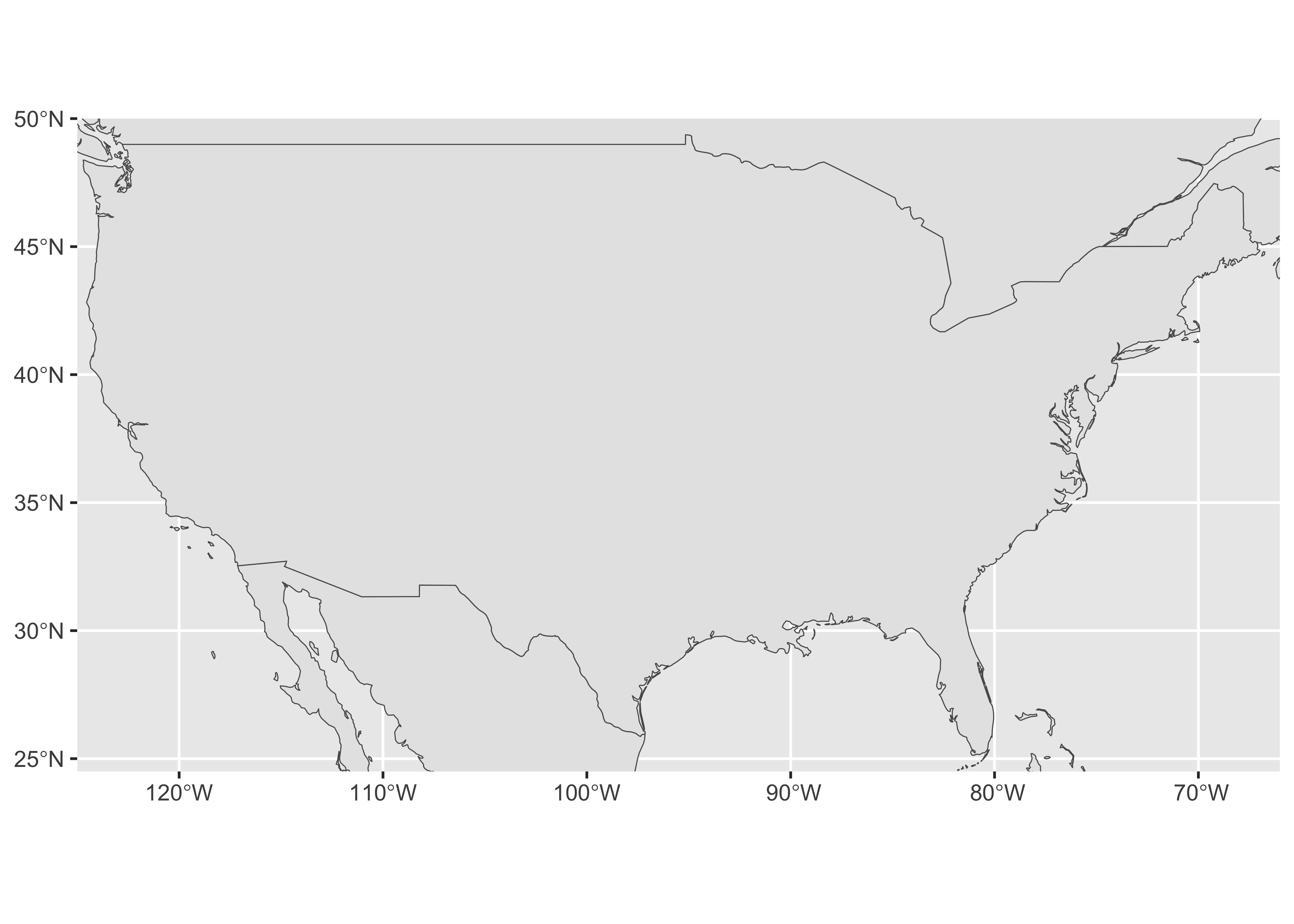

Monitor Data

Adding in our monitors…

ggplot(data = world) +
    geom_sf() +
    coord_sf(xlim = c(-125, -66), ylim = c(24.5, 50), 
             expand = FALSE)+
    geom_point(data = pm, aes(x = lon, y = lat), size = 2, 
               shape = 23, fill = "darkred")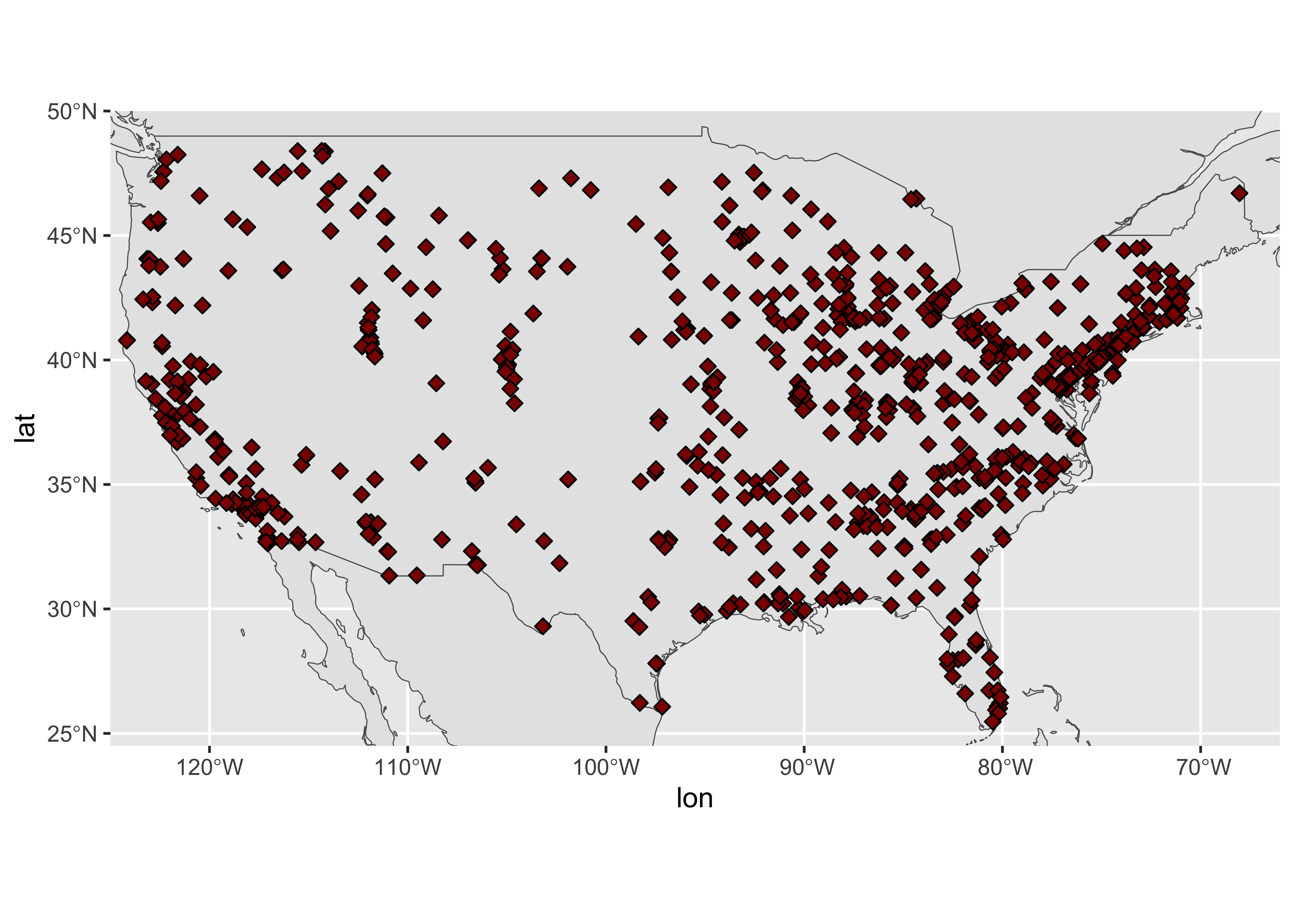

County Lines

Adding in county lines

counties <- sf::st_as_sf(maps::map("county", plot = FALSE,
                                   fill = TRUE))

counties

Simple feature collection with 3076 features and 1 field
Geometry type: MULTIPOLYGON
Dimension:     XY
Bounding box:  xmin: -124.6813 ymin: 25.12993 xmax: -67.00742 ymax: 49.38323
Geodetic CRS:  +proj=longlat +ellps=clrk66 +no_defs +type=crs
First 10 features:
                               ID                           geom
alabama,autauga   alabama,autauga MULTIPOLYGON (((-86.50517 3...
alabama,baldwin   alabama,baldwin MULTIPOLYGON (((-87.93757 3...
alabama,barbour   alabama,barbour MULTIPOLYGON (((-85.42801 3...
alabama,bibb         alabama,bibb MULTIPOLYGON (((-87.02083 3...
alabama,blount     alabama,blount MULTIPOLYGON (((-86.9578 33...
alabama,bullock   alabama,bullock MULTIPOLYGON (((-85.66866 3...
alabama,butler     alabama,butler MULTIPOLYGON (((-86.8604 31...
alabama,calhoun   alabama,calhoun MULTIPOLYGON (((-85.74313 3...
alabama,chambers alabama,chambers MULTIPOLYGON (((-85.59416 3...
alabama,cherokee alabama,cherokee MULTIPOLYGON (((-85.46812 3...

monitors <- ggplot(data = world) +
    geom_sf(data = counties, fill = NA, color = gray(.5))+
      coord_sf(xlim = c(-125, -66), ylim = c(24.5, 50), 
             expand = FALSE) +
    geom_point(data = pm, aes(x = lon, y = lat), size = 2, 
               shape = 23, fill = "darkred") +
    ggtitle("Monitor Locations") +
    theme(axis.title.x=element_blank(),
          axis.text.x = element_blank(),
          axis.ticks.x = element_blank(),
          axis.title.y = element_blank(),
          axis.text.y = element_blank(),
          axis.ticks.y = element_blank())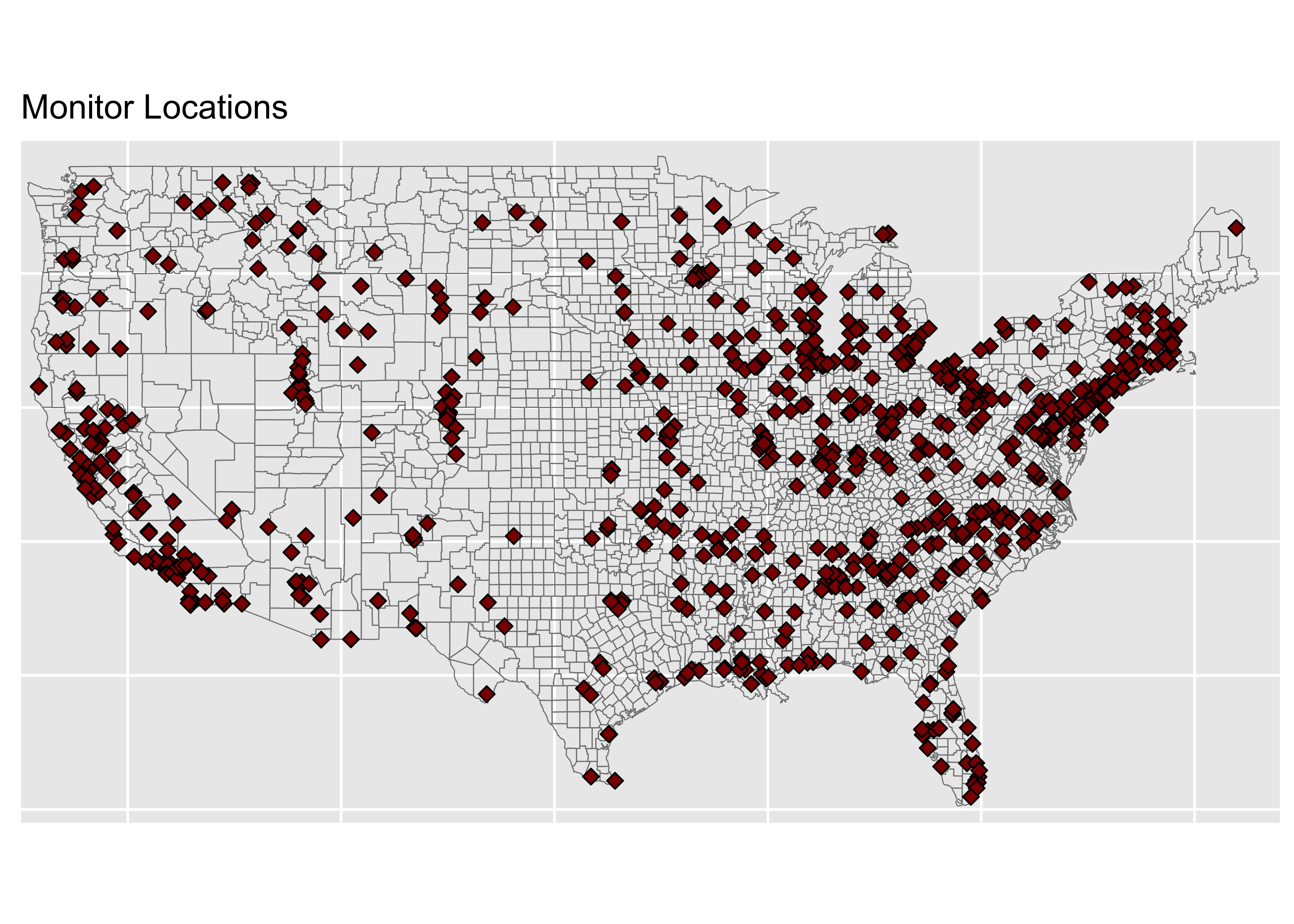

Counties

Wrangle counties:

separate county and state into separate columns
make title case
combine with PM data

counties <- counties |> 
  tidyr::separate(ID, into = c("state", "county"), sep = ",") |> 
  dplyr::mutate(county = stringr::str_to_title(county))

map_data <- dplyr::inner_join(counties, pm, by = "county")

Map: Truth

Code
Plot

truth <- ggplot(data = world) +
  coord_sf(xlim = c(-125,-66),
           ylim = c(24.5, 50),
           expand = FALSE) +
  geom_sf(data = map_data, aes(fill = value)) +
  scale_fill_gradientn(colours = topo.colors(7),
                       na.value = "transparent",
                       breaks = c(0, 10, 20),
                       labels = c(0, 10, 20),
                       limits = c(0, 23.5),
                       name = "PM ug/m3") +
  ggtitle("True PM 2.5 levels") +
  theme(axis.title.x = element_blank(),
        axis.text.x = element_blank(),
        axis.ticks.x = element_blank(),
        axis.title.y = element_blank(),
        axis.text.y = element_blank(),
        axis.ticks.y = element_blank())

Coordinate system already present. Adding new coordinate system, which will
replace the existing one.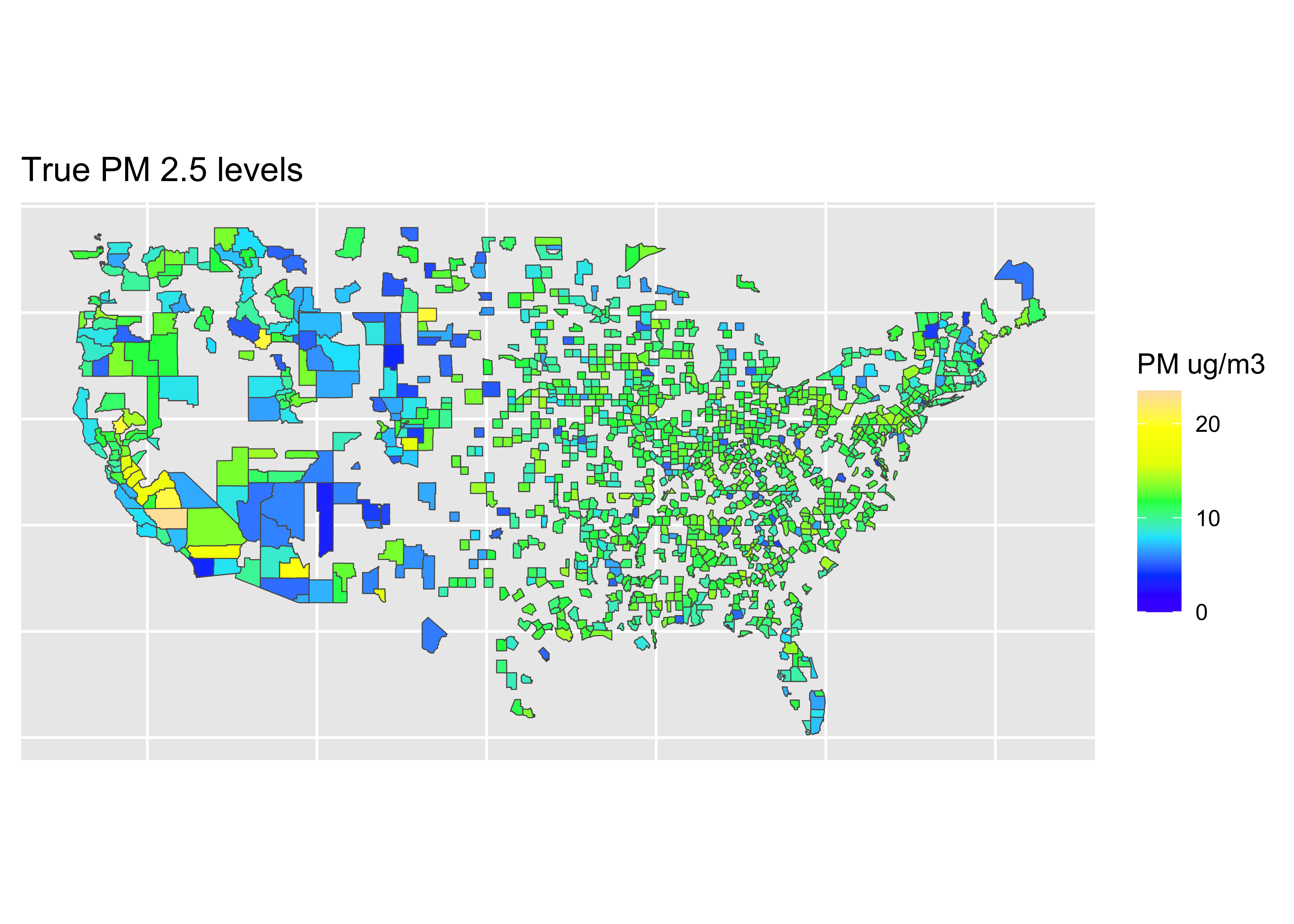

Map: Predictions

# fit data
RF_final_train_fit <- parsnip::fit(RF_tuned_wflow, data = train_pm)
RF_final_test_fit <- parsnip::fit(RF_tuned_wflow, data = test_pm)

# get predictions on training data
values_pred_train <- predict(RF_final_train_fit, train_pm) |> 
  bind_cols(train_pm |> select(value, fips, county, id)) 

# get predictions on testing data
values_pred_test <- predict(RF_final_test_fit, test_pm) |> 
  bind_cols(test_pm |> select(value, fips, county, id)) 
values_pred_test

# A tibble: 292 × 5
   .pred value fips  county     id       
   <dbl> <dbl> <fct> <chr>      <fct>    
 1  11.6  11.2 1033  Colbert    1033.1002
 2  11.9  12.4 1055  Etowah     1055.001 
 3  11.1  10.5 1069  Houston    1069.0003
 4  13.9  15.6 1073  Jefferson  1073.0023
 5  12.0  12.4 1073  Jefferson  1073.1005
 6  11.3  11.1 1073  Jefferson  1073.1009
 7  11.5  11.8 1073  Jefferson  1073.5003
 8  11.0  10.0 1097  Mobile     1097.0003
 9  11.9  12.0 1101  Montgomery 1101.0007
10  12.9  13.2 1113  Russell    1113.0001
# ℹ 282 more rows

# combine
all_pred <- bind_rows(values_pred_test, values_pred_train)

map_data <- inner_join(counties, all_pred, by = "county")

pred <- ggplot(data = world) +
  coord_sf(xlim = c(-125,-66),
           ylim = c(24.5, 50),
           expand = FALSE) +
  geom_sf(data = map_data, aes(fill = .pred)) +
  scale_fill_gradientn(colours = topo.colors(7),
                       na.value = "transparent",
                       breaks = c(0, 10, 20),
                       labels = c(0, 10, 20),
                       limits = c(0, 23.5),
                       name = "PM ug/m3") +
  ggtitle("Predicted PM 2.5 levels") +
  theme(axis.title.x=element_blank(),
        axis.text.x=element_blank(),
        axis.ticks.x=element_blank(),
        axis.title.y=element_blank(),
        axis.text.y=element_blank(),
        axis.ticks.y=element_blank())

Coordinate system already present. Adding new coordinate system, which will
replace the existing one.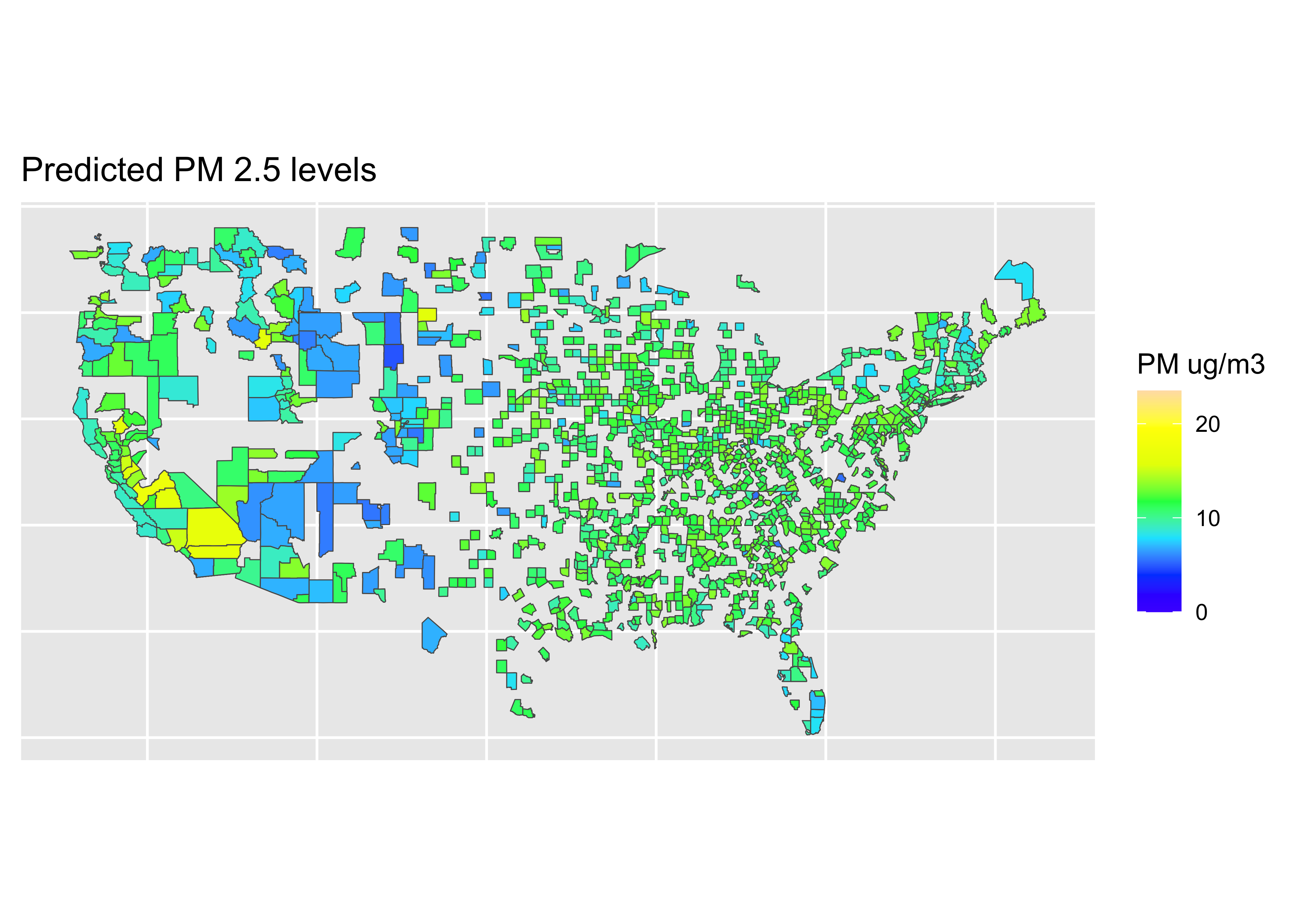

Final Plot

:::panel-tabset

Code

library(patchwork)

final_plot <- (truth/pred) + 
  plot_annotation(title = "Machine Learning Methods Allow for Prediction of Air Pollution", subtitle = "A random forest model predicts true monitored levels of fine particulate matter (PM 2.5) air pollution based on\ndata about population density and other predictors reasonably well, thus suggesting that we can use similar methods to predict levels\nof pollution in places with poor monitoring",
                  theme = theme(plot.title = element_text(size =12, face = "bold"), 
                                plot.subtitle = element_text(size = 8)))

Plot

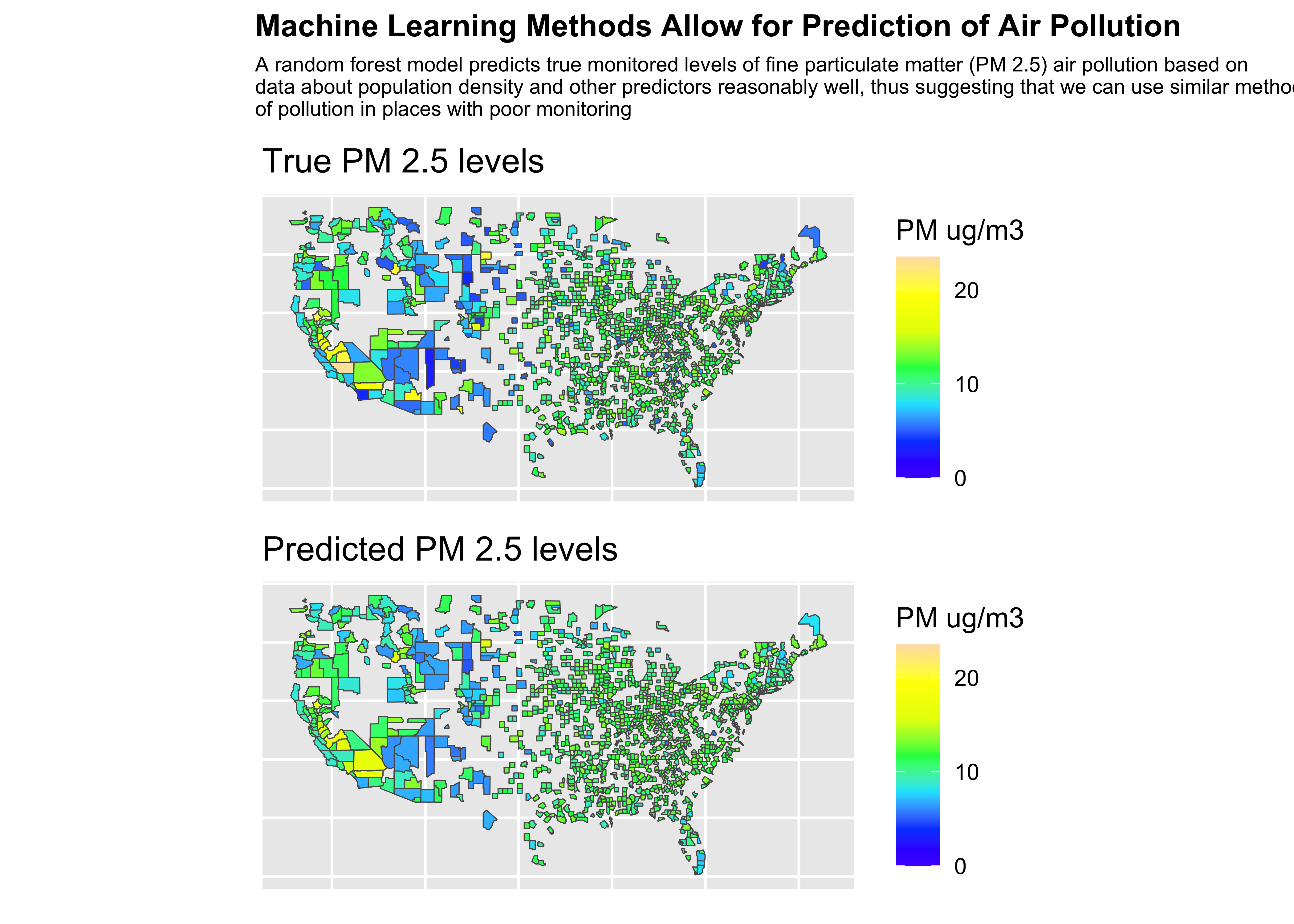
❓ What do you learn from these results?

Your Case Study

Can you copy + paste code directly from here to answer the question? Yes.
Do you have to present linear regression model and random forest? No
Should you present anything from the 12-regression notes? Probably not. (This is why HW03 and lab07 focus on regression)
Could you try an additional model as your extension? Yes!
Does that model have to be “better”? No! But, consider the story!
Could you try to identify the simplest, accurate model as an extension? Yes.

CS02: Predicting Air Pollution (Analysis)

Q&A

Course Announcements

Progress Check-in

Question

Analysis

Building our tidymodels knowledge:

The Data

Data Splitting

Split the Data

Pre-processing: recipe() + bake()

Step 1: Specify variable roles

Step 2: Pre-process with step*()

Steps

Selecting Variables

One-hot Encoding

Putting our recipe together

Step 3: Running the pre-processing (prep)

Step 4: Extract pre-processed training data using bake()

Step 5: Extract pre-processed testing data using bake()

Aside: return to wrangling

Specifying our model (parsnip)

Step 1: Specify the model

Step 2: Fit the model

Step 3: Prepare the recipe (estimate the parameters)

Step 4: Assess model fit

Visualizing Model Performance

Quantifying Model Performance

Cross-Validation

Implementing in rsample()

Model Assessment on v-folds

A different model?

Random Forest

[source]

But not just one tree…

Visualizing a RF

Updating our recipe()

Model Specification

Workflow

Fit the Data

Assess Feature Importance

Assess Model Performance

Model Tuning

Check Metrics:

Final Model Evaluation

Visualizing our results

A map of the US

Outline of the US

World map:

Just the US

Just the US

Monitor Data

County Lines

The Map

Counties

Map: Truth

Map: Predictions

Final Plot

Code

Plot

Your Case Study

Building our `tidymodels` knowledge:

Pre-processing: `recipe()` + `bake()`

Step 2: Pre-process with `step*()`

Putting our `recipe` together

Step 3: Running the pre-processing (`prep`)

Step 4: Extract pre-processed training data using `bake()`

Step 5: Extract pre-processed testing data using `bake()`

Specifying our model (`parsnip`)

Implementing in `rsample()`

Updating our `recipe()`